

Abstract
Accurate quantification of forest carbon stocks and fluxes over regions is needed to monitor forest resources as they respond to changes in climate, disturbance and management, and also to evaluate contributions of forest sector to the regional and global carbon balances. In previous work we introduced a national forest carbon monitoring system (NFCMS) that combines forest inventory data, satellite remote sensing of stand biomass and forest disturbances, and an ecosystem carbon cycle model to assess contemporary forest carbon dynamics at a 30 m resolution. In this study, we evaluate the NFCMS estimates of biomass and carbon fluxes with available data products for the Pacific Northwest (PNW) region, and then analyze the regional carbon balance over the period 1986–2010. The biomass estimates have good agreements with evaluation datasets (eMapR, NBCD2000, and Hagen2005) at regional and forest type levels, and at spatial scales of 1 km2 and larger. Regionwide, PNW forests acted as a stable net sink for atmospheric CO2 (18.5 Tg C yr–1) within forestlands. However, harvesting activities removed significant amounts of carbon, equating to over 75% of annual net carbon sink, though only 25% of this (∼3.5 Tg C yr–1) is emitted to the atmosphere within 50 years. Wildfires contributed modestly to carbon emissions in most years, however, the severe fires of 2002 and 2006 released 16.6 and 7.1 Tg C, respectively. The study demonstrates the potential of the NFCMS framework to serve as a candidate measuring, reporting and verification system, informed by field and remotely sensed inventories, and tracking the carbon balance of the forest sector across the United States.
Export citation and abstract BibTeX RIS

Original content from this work may be used under the terms of the Creative Commons Attribution 4.0 license. Any further distribution of this work must maintain attribution to the author(s) and the title of the work, journal citation and DOI.
1. Introduction
Forests play an important role in the coupled carbon-climate system by storing carbon (Bonan 2008), and have helped to slow down climate change by absorbing about one-quarter of the carbon emitted by human activities (King et al 2007, Domke et al 2018, Keenan and Williams 2018). As such, forest carbon sequestration is one of several natural climate solutions that have great potential to contribute to negative carbon emissions pathways (Stocker et al 2013, Fargione et al 2018). At the same time, many of the world's forests are being intensively managed to meet humanity's needs for timber, fiber, and other ecosystem services. For example, timber harvesting removes ∼0.13 Pg C yr−1 from US forestlands (EPA 2011), resulting in similarly large carbon releases to the atmosphere that offset a sizeable portion the net carbon uptake in US forestlands. Therefore, it is crucial that we develop robust measuring and monitoring systems to document changes in global forest resources, the underlying drivers of these changes, and their implications for climate and society.
Aboveground live woody biomass (AGB) is one of the largest stores of carbon in forest ecosystem, reflecting important aspects of the health and environmental conditions of a forest. Monitoring systems have tended to focus on AGB because it is readily measured both in situ and remotely. Field-based forest inventories provide valuable records of forest live and dead biomass, as well as many more characteristics and determinants of forest carbon stocks including forest species composition, disturbance history, and management attributes (Birdsey 1992, Smith and Heath 2002, Jenkins et al 2003). While enormously valuable, the long interval between measurements (∼5–10 years), sparse spatial sampling with limited coverage, and regional/national variability in inventory methods challenge large area assessments of carbon stock variability over time and space (Masek and Collatz 2006). Various remote sensing platforms offer unified and consistent forest carbon assessments, and have been widely used to quantify biomass carbon stocks at regional to global scales since the early 1990s. Remote sensing is a cost-effective tool to provide the spatiotemporally continuous mapping of forests. Recent advances in remote sensing, including passive optical remote sensing, microwave remote sensing, and light detection and ranging (LiDAR; e.g. Lefsky et al 2005, Nelson et al 2009), opened a new window on monitoring forest AGB and its change over time. Biomass cannot be directly measured from these remote observations, but the information detected by various sensors can be used to estimate forest AGB, particularly when coupled with plot-level forest inventory that guide AGB mapping with empirical algorithms or machine learning methods (e.g. Powell et al 2010, Gleason and Im 2012, Li et al 2020). Multiple biomass products have been generated across a range of spatial extents, from local and regional to global scales in recent years, but most offer a snapshot account at a given moment in time (e.g. Saatchi et al 2011). Recently, Kennedy et al (2018) produced the first annual forest biomass product for the conterminous United States from 1984 to 2017. Kennedy's dataset assigns field-measured biomass from the USFS forest inventory and analysis (FIA) program to 30 m pixels with an empirical method based on the biophysical similarity between these two scales.
Biomass observations, on their own, provide an incomplete account of forest carbon stock and flux dynamics and their contributions to emissions and removals of atmospheric CO2. What is also needed is an account of the fate of biomass removals, whether involving direct combustion emissions from wildfires, on-site decay from disturbance-induced mortality and decomposition, or harvest removal with a range of fates throughout the wood products sector (Williams et al 2016, Domke et al 2018, Hurtt et al 2019). Extending from biomass change to carbon flux dynamics and balance of forest ecosystems, and of the whole forest sector, requires integration with broader carbon accounting frameworks (e.g. Gu et al 2019). This typically involves models that can assess how changes in biomass are related to other ecosystem carbon pools (e.g. dead wood and soil carbon) as they change over time, and also throughout the wood products sector (e.g. fuelwood, paper, building materials, or stored as waste).
Previous studies have shown poor agreement between satellite-measured biomass and model-derived biomass in forests (e.g. TRENDY v6 DGVMs in Yang et al 2020), and large uncertainties exist among several model-derived biomass datasets (e.g. Friend et al 2014, Ahlström et al 2017). To improve model-based estimates, our previous studies proposed a framework to utilize the stand age-biomass relationships from FIA measurements and fit these trajectories into the biogeochemical model. The time series of forest carbon stocks are estimated by combining information from earth-observing satellite data on forest biomass and disturbance, field data from the FIA program, and a carbon cycle model in our national forest carbon monitoring system (NFCMS; Williams et al 2012, 2014, Gu et al 2016). The system calculates carbon accumulation in biomass from growth, declines associated with disturbances, and the storage or release fate within a process-based framework. It is designed to report the change in forest net carbon exchange with the atmosphere as well as net biome productivity, both of which are essential components in the assessment of forest sector contributions to atmospheric CO2 concentration and are critical for Tier 3 measuring, reporting, and verification (MRV) in assessing forest carbon sequestration and emission with the long-term and spatially explicit data to obtain greater certainty (IPCC 2006, 2019). This study builds upon our prior work by providing detailed illustrations of the local scale carbon dynamics for select regions of interest (ROIs) to demonstrate the capacity of the NFCMS to provide information for decision makers at a scale relevant to land managers and not just for state-level to continental scale carbon monitoring and reporting. The objectives of this study are (a) to evaluate annual forest AGB derived from our NFCMS framework with comparison to other data products, (b) to demonstrate the framework's utility for local to continental scale MRV of the forest sector informing land managers concerned with timber production, forest conservation, and regional carbon balance, and (c) to examine the ability of this technique to track forest carbon stock and flux dynamics within local patches in several disturbed scenarios that is relevant for land managers and other decision makers. This study is the first in our series that formally evaluates the biomass time series we obtain from the NFCMS approach with comparison to available datasets and at a range of scales.
2. Data and methods
2.1. NFCMS framework
The overarching method (figure 1) involved (a) the training of a forest carbon cycle model, the Carnegie-Ames-Stanford Approach (CASA) model (figure S1 (available online at stacks.iop.org/ERL/16/055026/mmedia); Potter et al 1993, Randerson et al 1996), to match biomass accumulation with stand development (henceforth referred as stand age) from the FIA data, and the use of that trained model to calculate carbon stocks and fluxes with stand age for each possible combination of forest-type, productivity level, pre-disturbance conditions, and disturbance type, (b) the determination of pixel‐level characteristics for all forested pixels across the Pacific Northwest (PNW) United States at a 30 m resolution, and the assignment of stand age, carbon stocks and fluxes for each 30 m forested pixels according to its specific attributes, and (c) the estimate of regional carbon stock balance, carbon stock potentials and emission risks using the WoodCarb II model (Skog 2008). The NFCMS methodology is briefly described here and more fully detailed in Supplement and prior works (Williams et al 2012, 2014, Gu et al 2016, 2019).

Figure 1. Flowchart of national forest carbon monitoring system (NFCMS).
Download figure:
Standard image High-resolution imageThe CASA model parameters, including production (Pw)-related parameters and wood turnover rate (Aw), were adjusted to best match modeled aboveground wood production with the biomass accumulation in the FIA forest inventory data for each combination of forest-type group and low and high site productivity classes (Williams et al 2012). To encompass the range of AGB-age variances, 20 curves were generated for each case from age one to the maximum stand age recorded in the FIA database. The CASA model was also altered to capture disturbance impacts on the carbon cycle, by imposing a forest disturbance during the spin-up phase of the simulations (Williams et al 2014). After spin-up, simulations were run for either harvest or fire disturbances. Harvest disturbances are simulated by killing 80% of the biomass in live pools, removing a large proportion of the aboveground wood biomass from site as harvested wood, and re-allocating the remaining killed biomass to decompose on-site in their respective carbon pools of litter, coarse woody debris (CWD) and soil pools (see supplement for details). Fire disturbances were simulated by applying mortality and consumption rates for three different fire intensity levels as developed by Ghimire et al (2012). We saved the AGB-age trajectories and the net ecosystem productivity (NEP)-age trajectories for each simulation.
The forests attributes considered in our framework for each 30 m resolution forested pixels are forest-type groups (Ruefenacht et al 2008), site productivity class (from the method in Williams et al 2014), stand age, pre-disturbance biomass class as well as disturbance type. The stand age for each pixel is inferred as the age on the CASA age-biomass curves corresponding to the biomass reported in the NACP Aboveground Biomass Carbon Dataset in the year 2000 (NBCD2000; Kellndorfer et al 2000, 2013) for that pixel and adjusted to account for forest disturbances and regrowth before and after 2000 according to the North American Forest Dynamics dataset (NAFD; Goward et al 2016) and Monitoring Trends in Burn Severity (MTBS; Eidenshink et al 2007). Disturbance type was assigned to fire for pixels marked as MTBS events and to harvest for pixels marked in NAFD. For all forests with disturbances prior to year 2000, pre-disturbance biomass was estimated as the biomass values of undisturbed forests of same forest-type averaged over a local grid of 1 km, widened to 10 km if it remained undefined at the 1 km scale. For all 'undisturbed forest' in NAFD, pre-disturbance biomass was estimated as the average biomass of same forest-type and productivity class over the entire region. The combination of all pixel-specific attributes allowed us to calculate statistics of AGB and NEP for each year at the pixel-level from 1986 to 2010, including median and standard deviation, based on the sampling of AGB-age and NEP-age curves, respectively.
In addition to AGB and NEP, we also trace the fate of carbon removed from forests by harvest with the WoodCarb II model (Skog 2008). Our prior work (Gu et al 2016) did not track the fate of harvested wood products (HWPs) with a detailed modeling and that this new addition offers a critical advance needed for assessing the net CO2 exchange between the forest sector and the atmosphere. Using data from the USDA Forest Service timber product output online database (USDA 2012), we estimated the forest-type specific proportion of wood entering each of the 14 HWP categories of the WoodCarb II model as well as the two categories of 'fuelwood' and 'other removals' that do not enter the HWP stream and are assumed to release their carbon directly to the atmosphere in the year of harvest. For each year after harvest, WoodCarb II uses exponential decay functions with HWP-category specific half-life values to calculate the proportion of wood that remains in use in each category, the rest being either burned, composted or discarded in solid waste disposal sites (SWDS). Carbon in SWDS is either stored indefinitely or decomposed following another exponential decay function and released to the atmosphere as either carbon dioxide or methane. More details can be found in the supplement section 1.3. To assess the regional carbon balance, carbon stock potential, and emissions risks, we inferred the committed emissions of harvest removals over 50 years to represent harvest emission.
While this framework has been applied nationwide (https://doi.org/10.3334/ORNLDAAC/1829), this study focuses on the PNW region (section 2.3) as a case study to evaluate NFCMS-estimated AGB and carbon flux and balance dynamics with comparison to other spatially-extensive datasets that are readily available at this time.
2.2. Evaluating NFCMS-estimated forest carbon
We compared NFCMS-estimated AGB to annual forest AGB maps generated by the eMapR research group at Oregon State University (eMapR biomass, Kennedy et al 2018) with a temporal coverage spanning from 1984 to 2017. The eMapR biomass used FIA plot-level aboveground live wood biomass, statistical modeling, and time-series of satellite images. Landsat data are analyzed through LandTrendr (Kennedy et al 2010) to create disturbance maps, change agent maps, and temporally-stabilized yearly image time-series. Rather than building biomass-age models as adopted in the NFCMS method, eMapR biomass was derived with gradient nearest neighbor (GNN) imputation, assigning FIA-measured biomass to pixels which have similar spectral characters, climatic settings, and geospatial characteristics in comparison to the FIA plot settings (Ohmann et al 2014, Kennedy et al 2018). GNN algorithm used spectral variables derived from the temporally-stabilized yearly imagery mosaics generated by LandTrendr.
In addition, we compared NFCMS results to two single-year AGB maps. The first is NBCD2000, representing AGB at 30 m resolution across the conterminous US. This data set used an empirical modeling approach (regression tree) that combined FIA biomass data with high-resolution InSAR data acquired from the 2000 Shuttle Radar Topography Mission and optical remote sensing data acquired from the Landsat ETM+ sensor (Kellndorfer et al 2000, 2013). The second is from Hagen et al (2016) (Hagen2005), representing the AGB status in 2005. This data set is based on inventory data and Geoscience Laser Altimeter System (GLAS) Lidar data. Canopy height characteristics, such as percentile of energy and waveform extent, were derived from more than 450 000 clean GLAS Lidar. To relate forest height to biomass, combined height metrics were calibrated with Lorey's height (basal area weighted height) from ground measurements (Lefsky 2010, Healey et al 2012). AGB was estimated with the equivalent of Lorey's height derived from GLAS full waveform Lidar data. Estimates were calibrated with ground inventory data from plots located approximately under the Lidar footprint in needleleaf, broadleaf, and mixed forests (Lefsky 2010).
We firstly compared the NBCD2000 with NFCMS in 2000 for the undisturbed forests to test the robustness of our method in reproducing the biomass map in 2000. We used an integrated disturbance map from NAFD and MTBS for statistical analyses. This map indicates the year of disturbance and type of disturbance (harvest and fire). Areas considered to be forested were all locations for which both the NFCMS and the eMapR datasets report AGB exceeding 0.1 kg C m−2 for at least one year during 1986–2010. We calculated temporal profiles of forest biomass from two time series datasets (i.e. NFCMS and eMapR), including median and standard deviation, and their correlation coefficient (r) and root mean square error (RMSE) of yearly means. We compared the region-wide averages between NFCMS and evaluating datasets, as well as the biomass agreement over a range of spatial scales from the original 30 m to an aggregation as coarse as ∼40 km. At each spatial scale (e.g. 3 km), we randomly selected 500 samples that only included forested pixels (e.g. 1000 × 1000, 30 m pixels) and aggregated these to the target scale. We calculated the RMSE of these 500 random samples between two biomass datasets to represent their agreement.
We selected several ROIs which have different disturbance histories to compare the differences between two temporally continuous products (i.e. NFCMS and eMapR) for total AGB, for those that have not experienced a stand-replacing disturbance from 1986 to 2010 according to the NAFD dataset, and for those that experienced disturbances (harvest and fire) from 1986 to 2010. Also, we examined the corresponding changes in NEP before and after forest disturbances as estimated by the NFCMS framework.
2.3. Study area
The PNW region includes Washington and Oregon states. The dominant forest types are Douglas-fir (48.6%), Ponderosa pine (17.0%), and Fir/Spruce/Mountain Hemlock group (15.1%; figure 2(a)). The forests in the PNW region encompass an enormous range of climatic and physiographic variabilities, but can be broadly classified into two geographic regions: a moist zone located west of the crest of the Cascade mountain range, and a dry zone located east of the Cascade crest in southwestern Oregon (Franklin and Johnson 2012, Wimberly and Liu 2014). The moist zone has a Mediterranean climate characterized by relatively cool wet winters and warm dry summers with most precipitation falling as rainfall except at the highest elevation (figure S7). The dry zone has a more continental climate generally characterized as having colder winters, hotter summers, and low precipitation with a high proportion occurring as snow. Various kinds of forest disturbances occur in the PNW region, including both human disturbance (e.g. timber harvest) and natural disturbance (e.g. fire, insect, wind, and flooding) (figures 2(b) and (c)). About half (52%) of all harvesting occurred in Douglas-fir forests, followed by Ponderosa Pine (20%), Fir/Spruce/Mountain Hemlock (8%), and Hemlock/Sitka Spruce (7%). Of all forestlands that burned, 37% was in Douglas-fir stands, 27% in Ponderosa Pine, and 21% in Fir/Spruce/Mountain Hemlock. Historical fire regimes in these moist forests were characterized by large, high severity fires with long return intervals (200–500 years), although fire regimes in some parts of the moist forest zone were mixed-severity with shorter return intervals (Agee 1996, Long and Whitlock 2002, Weisberg and Swanson 2003). Other important disturbances in western Oregon and Washington typically result from winter storm events with high wind and precipitation and include flooding. In this study, we focused on the harvest and fire impact as they accounted for the largest percentage among all agents in the period of 1986–2010.
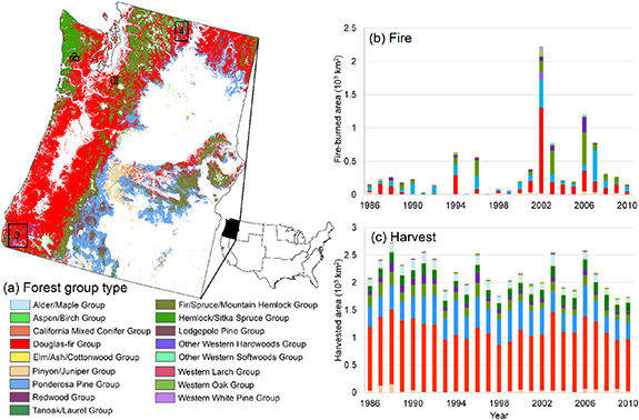
Figure 2. (a) Map of forest group type in the Pacific Northwest (PNW) region and the time-series of (b) burned and (c) harvested areas of each forest group from 1986 to 2010. Four regions of interest (ROIs) are shown by the boxes in panel (a).
Download figure:
Standard image High-resolution image3. Results
3.1. Evaluation of NFCMS-estimated biomass
The spatially-averaged, overall temporal pattern of AGB estimates from NFCMS and eMapR agree well in recently undisturbed forests (RUFs) in the PNW region (r = 0.96, RMSE = 0.52 kg C m–2; figure 3(a)). NFCMS has slightly higher estimates than eMapR after 2002. AGB significantly increased from 1986 to 2010 in the RUFs at a rate of 0.11 kg C m–2 yr–1 (level of statistical significance p < 0.01) from NFCMS estimates and 0.08 kg C m–2 yr–1 (p < 0.01) from eMapR. The NBCD2000 (10.9 kg C m–2) have a comparably better agreement with NFCMS (10.7 kg C m–2) in the RUFs (figure 3(b)) than eMapR (10.4 kg C m–2), which is also expected because NFCMS used undisturbed NBCD2000 AGB as the baseline for its time-series mapping. We see similarly good agreement when comparing maps of NBCD2000 and NFCMS in 2000 for RUFs (figure S8). NFCMS also agrees well with Hagen2005 in the year 2005, both indicating an average AGB of 11.4 kg C m–2, while eMapR indicated 10.7 kg C m–2.
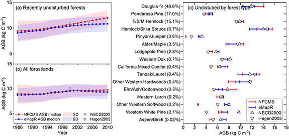
Figure 3. Comparison of annual biomass estimates derived from NFCMS, eMapR, NBCD2000, and Hagen2005 for (a) recently undisturbed forests and for (b) all forestlands in the PNW region, and (c) by forest type in recently undisturbed areas. The bar in panel (c) represents interannual range of AGB medians derived from NFCMS (red) and eMapR (blue). The ranking is based on the proportion of each forest type in total forestlands, with the proportion shown in the parentheses after each forest type group name.
Download figure:
Standard image High-resolution imageSimilarly, for all forestlands, time-series from NFCMS and eMapR have good agreement in annual AGB which RMSE is 0.28 kg C m–2 and in long-term trend from 1986 to 2010 (r = 0.88, figure 3(b)). Both NFCMS and eMapR present slightly lower biomass estimates in 2000 and 2005 compared to the NBCD2000 and Hagen2005 (10.0 and 9.9 kg C m–2, respectively) when comparing across all forestlands, including those areas that experienced significant disturbances. Logically, the subtle increase in departures between NFCMS/eMapR and NBCD2000/Hagen2005 can be attributed to recently disturbed areas. AGB estimates from NFCMS (9.3 ± 0.33 kg C m–2 yr–1) and eMapR (9.2 ± 0.31 kg C m–2 yr–1) are both fairly stable over the 25 year period when averaged across all forestlands in the PNW region. This indicates that AGB losses due to disturbance events nearly offset the AGB increases in the areas that have been recently free of major disturbance.
Biomass estimates show close correspondences between NFCMS and these evaluation datasets across the most abundant forest types, including Douglas-fir, Ponderosa pine, Fir/Spruce/Mountain Hemlock, and Hemlock/Sitka Spruce (figure 3(c)). NFCMS has similar estimates compared to the eMapR AGB in some forest types that account for small proportions (<5%), but comparably lower estimates from NFCMS are presented in Pinyon/Juniper, Lodgepole Pine, other Western Softwood, and Aspen/Birch.
Datasets disagree at the original 30 m resolution, with RMSEs ranging between 3 and 5 kg C m–2 (figure 4). However, RMSEs drastically decline to less than 1.5 kg C m–2 when the spatial scale of aggregation is coarsened to 1 km, and they continue to decrease to about 1 kg C m−2 at the 5 km scale. These four AGB datasets show good and stable agreement at the spatial scale from 5 km to 30 km, with RMSEs within 1 ± 0.2 kg C m–2. This indicates that NFCMS has a similar ability (p < 0.01) in representing the biomass stock to the estimates from eMapR, NBCD2000, and Hagen2005 within these spatial scales that are greater than 1 km.
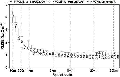
Figure 4. RMSEs of NFCMS biomass estimates and evaluation datasets across spatial scales. Solid circles represent the mean of yearly RMSEs from 1986 to 2010, and whiskers are the 1% and 99% quantiles.
Download figure:
Standard image High-resolution image3.2. Annual carbon balance in the PNW forest
NFCMS indicates that the three dominant forests types contribute strong carbon sinks (figure 5(a)), including Douglas-fir at around 200 g C m–2 yr–1 for recently undisturbed areas and total areas, followed by Hemlock/Sitka Spruce (164.1 and 146.2 g C m–2 yr–1 for the RUFs and total areas, respectively) and Fir/Spruce/Mountain Hemlock (66.5 and 60.2 g C m−2 yr−1 for the RUFs and total areas, respectively). Ponderosa pine, however, shows a weak carbon sink in its RUFs (32.0 g C m–2 yr–1). Other less common forest types, such as Tanoak/Laurel, Elm/Ash/Cottonwood, and Alder/Maple, also sequestrate large amounts of carbon per unit area. Most forest types presented a net carbon sink in 1986–2010, except for western white pine that experienced severe burning in 2002 and 2006. The fire impacts are further analyzed in two ROIs in section 3.3.
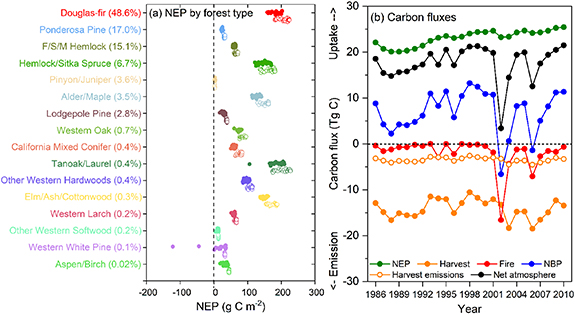
Figure 5. (a) Point clusters of yearly net ecosystem productivities (NEPs) for 1986–2010 averaged for each forest type in their recently undisturbed stands (hollow circles) and for all stands (solid dots), and (b) time-series of annual carbon fluxes between forests and the atmosphere (NEP) in the PNW region, along with harvest removals (Harvest) and fire (Fire) emissions, net biome productivity (NBP = NEP − harvest − fire), committed emissions of harvest removals over 50 years (harvest emissions), and between the atmosphere and forest sector (net atmosphere = NEP − harvest emissions − fire).
Download figure:
Standard image High-resolution imageOverall, forest ecosystems in the PNW region served as a stable net sink for atmospheric carbon, annually sequestrating about 18.5 Tg C from 1986 to 2010 (figure 5(b)). Annual NEP increased significantly at a rate of 0.20 Tg C yr–1 (p < 0.01), mainly due to a decrease in harvesting in the 1990s to early 2000s (figure 2(c)). Harvest removals range from 10.6 to 18.5 Tg C in 1986–2010 (table S1), and equate to more than 75% of the annual NEP. Cumulated emission from HWPs over 50 years accounts for 25% of harvest removals, ranging from 2.6 to 4.6 Tg C, while most of harvest removals remain in construction (34.3%) or are stored in SWDS (38.7%) at 50 years post-harvest (table S2; figure S6). The high proportion of carbon stored in products and SWDS is specific to the high proportion of softwoods harvested in the PNW region (table S1), including Douglas Fir, Hemlocks, Sitka Spruce, and Ponderosa Pines, which are preferentially used in longer-term uses. The large fluctuation of net biome productivity (NBP) resulted from large fire years, including 2002 and 2006, contributing emissions of 16.6 and 7.1 Tg C, respectively. These emissions pulses were so large that they changed the sign of NBP to be negative in these two years (–11.2 and −6.2 Tg C). Similarly, the full forest sector acted as a net carbon source to the atmosphere in 2002 (–1.3 Tg C) and saw much reduced net uptake in 2006 (7.7 Tg C) compared to other years (13.8 ± 1.9 Tg C).
3.3. Regional variations in forest carbon stock and flux due to harvesting and fire events
In an area with intensive and temporally variable harvesting (figure 6(a)), the temporal variations of biomass indicated by NFCMS and eMapR were found to be similar. Both NFCMS and eMapR present an increase in biomass in the RUFs from 1986 to 2010. The regionally averaged AGB is also consistent in these two datasets, showing a slight increase in 1986–2001 and then a decrease in 2002–2010, corresponding to the increased harvest within the latter period in this region. Moreover, NFCMS and eMapR have a good agreement in estimating the annual amount of harvest-killed biomass. Both datasets show a significant increase in annual harvest-killed biomass from 1986 to 2010 at rates of 4.6 × 10⁶ kg C yr–1 (p < 0.01) for NFCMS and 3.8 × 10⁶ kg C yr–1 (p < 0.01) for eMapR. Concurrently, the net carbon sink of the forestlands within this region decreased at a rate of −2.2 g C m–2 yr–1 (p < 0.01). The net carbon sink in 1997–1999 is close to the carbon sink in the RUFs, indicating the carbon sink in the forest regrowth period offsets the within-forestland carbon release by harvesting events, noting that this does not account for carbon emissions offsite. The weaker carbon sink after 2002 corresponds to increased harvest and the associated decrease in primary productivity along with prompt carbon emissions of decomposing harvest-killed biomass after the harvest. The carbon sink in the early regrowth period is generally larger than old stands (figure S3), which eases the decreasing trend in NEP.
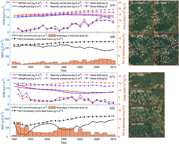
Figure 6. Comparison of AGB time-series from NFCMS and eMapR in (a) and (b) ROI 1 and (c) and (d) ROI 2 for which harvest is the major disturbance in 1986–2010, and the corresponding NEP variations for all forestlands and recently undisturbed forests. The satellite images in subpanels (b) (Google Earth 2019a) and (d) (Google Earth 2019b) show the temporal difference in land cover of each ROI. The images are Image Landsat/Copernicus provided by Google Earth Pro ©2021 Google.
Download figure:
Standard image High-resolution imageIn area where harvesting exhibited a decreasing trend (figures 6(c1)–(d4)), we find similar temporal trends from NFCMS and eMapR, although AGB is slightly higher for NFCMS than eMapR after 1992. Both NFCMS and eMapR indicate a decrease in harvest from 1986 to 2010 at the rates of −6.9 × 10⁵ kg C yr–1 (p = 0.1) and −2.0 × 10⁶ kg C yr–1 (p < 0.01), respectively. Similar to the increased harvest scenario in ROI 1, this region presented a weak net carbon sink due to the intensive harvesting events in 1987–1990 and 1997–2000 that accounted for 42% of the total area in this region. NEP of total forestland increased significantly at a rate of 11.7 g C m–2 yr–1 (p < 0.01) after 2000, and forest carbon sink increased rapidly to 186 g C m–2 in 2010 from 73 g C m–2 in 2000. This results from decreased harvest and regrowth in previously harvested lands. The fluctuation of NEP in ROIs 1 and 2 indicates its strong sensitivity to harvest timing and trend, and regrowing status.
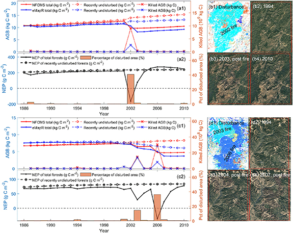
In two areas that experienced extensive wildfires (figure 7), NFCMS and eMapR generally show a good agreement in biomass estimates (total and recently undisturbed) before fire occurrences but present some disagreements after the fire, especially regarding the fire-killed biomass. NFCMS tends to have a higher fire-killed biomass estimate than the eMapR. In the 2002 fire, NFCMS estimates 8.9 × 10⁹ kg C of fire-killed biomass, which is about three times higher than eMapR (2.6 × 10⁹ kg C; figure 7(a1)). NFCMS also has a relatively high fire-killed biomass estimate in the 2006 fire in ROI 4 (figure 7(c1)). In addition to divergences in fire-killed biomass, AGB from eMapR presents a slight decline in the RUFs after the fire occurrences indicated by MTBS, unlike NFCMS. This mainly results from the fact that NFCMS uses the fire mask from MTBS dataset, which might have extra burned areas than the eMapR indicates in the year of fire occurrence, and eMapR identifies these areas as burned in the following years. eMapR uses Landsat spectral change to recognize the disturbance in LandTrendr, however, the fire charred post-burn environment can be as dark as forest in the Landsat visible spectral bands, which could lead to missing fire occurrences in these two regions. Another potential reason is that eMapR has other burned areas which are not shown in the MTBS map, explaining the decreasing biomass in areas that NFCMS would treat as undisturbed (figure 7(c1)).
Figure 7. Comparison of AGB time-series from NFCMS and eMapR in (a) and (b) ROI 3 and (c) and (d) ROI 4 for that experienced large fire events in 1986–2010, and the corresponding NEP variations for all forestlands and recently undisturbed forests. The satellite images in subpanels (b) (Google Earth 2019c) and (d) (Google Earth 2019d) show the land cover difference before and after the major fire events (indicated by MTBS) of each ROI. The images are Image Landsat/Copernicus provided by Google Earth Pro ©2021 Google.
Download figure:
Standard image High-resolution image
In addition to direct fire emissions from combustion, reductions in biomass production after severe fires (figure S4) plus decomposition of fire-killed biomass can lead to large carbon releases to the atmosphere in post-fire locations. This leads to a net carbon source in the case of severe burning where the NEP of ROI 3 is −164.3 g C m–2 in 2002 (figure 6(a2)) and the NEP of ROI 4 is −36.4 g C m–2 in 2006 (figure 7(c2)), and a weak net carbon sink post-fire with less severe burning (29.4 g C m–2 in 2003, figure 7(c2)). Ensuing regrowth leads to enhanced carbon sinks, but the speed of recovery to an NEP comparable to that of the RUFs depends on the regional forest productivity and fire severity.
4. Discussion
The NFCMS framework utilizes a process-based carbon cycle model trained by FIA AGB measurements in joint classes of forest type group, site productivity, and stand age, while the other data products rely on machine learning-based products applying empirical relationships in a way that is closer to a direct remote sensing approach. Disturbance-induced carbon stock changes in NFCMS are informed by a combination of disturbance maps from MTBS and NAFD. In contrast, eMapR infers disturbance impacts from temporal segmentation routines which can filter out some of the temporal dynamics (Kennedy et al 2018). Although NFCMS and eMapR disagree about the severity of wildfire killed biomass, the two datasets show similar temporal patterns in biomass changes and provide similar depictions of the impacts of disturbances on biomass stock at the regional scale. Moreover, we found good correspondence across data products at spatial scales of 1 km2 and larger despite major differences in methodologies. As expected, biomass comparisons at coarser resolution are more consistent than the original 30 m resolution, as shown in Huang et al (2017), with a prior evaluation of the eMapR biomass product indicating that the eMapR AGB may be less accurate at 30 m than when aggregated to broader scales (Kennedy et al 2018).
The annual aboveground carbon stock change in the PNW forests derived from NFCMS (1.4 Pg C yr–1) agrees well with FIA-derived estimates (1.7 Pg C yr–1) from Domke et al (2020) that relies on its own scaling from plots to landscapes. Large-area biomass assessments continue to be challenged by limited field data as well as wide variation in estimates across datasets. Various forest AGB data products are readily available across the globe (e.g. Saatchi et al 2011, Baccini et al 2017), but can show substantial differences (e.g. Huang et al 2019). Detailed accuracy assessment is challenged by the lack of appropriate reference data. True biomass product validation requires destructive harvesting, drying, and weighing of trees, though close approximations can be derived in the field with standard forest mensuration techniques. Field-based assessments of biomass stocks are invariably labor and time intensive presenting logistical challenges for developing extensive evaluation datasets and for repeat measurements. The extensive network of FIA plots provides an excellent base for a wide range of biomass mapping approaches, but it, too has shortcomings. For example, old trees and stands are uncommon and thus less well sampled, yet they can exhibit large variability in biomass and carbon stock conditions that may appear as biases in both the NFCMS and machine learning-based biomass estimation approaches (Kennedy et al 2018). In general, there is still a need for the generation of large AGB samples from in situ measurements to validate high-resolution passive remote sensing data (e.g. QuickBird, IKONOS, and UAVs) and lidar measurements. Duncanson et al (2019) noted that a community accepted standard for satellite-based biomass map validation is still lacking. The Committee on Earth Observing Satellites is developing a protocol to fill this need in advance of the next generation of biomass-relevant satellites, and Global Ecosystem Dynamics Investigation and BIOMASS mission that measure forest structure from spaceborne sensors might be able to facilitate future carbon stock benchmarking (Le Toan et al 2011, Stavros et al 2017, Reichstein and Carvalhais 2019, Xiao et al 2019).
With regard to net carbon sinks, NFCMS indicates an annual NEP in the PNW forests about 18.5 Tg C, also aligning well with the stock change-based estimates from the USFS (16.8 Tg C; Domke et al 2020). Moreover, both estimates show a trend of increased NEP in recent years. As forest aboveground woody biomass is one of the largest stores of carbon in the forest ecosystem and largely determines carbon exchange between forest and atmosphere (Baccini et al 2017), the good agreement between NFCMS-derived AGB and other datasets enables the confidence in estimated forest carbon sink. We find a stronger carbon sink in the PNW forest from this newer version comparing to the less advanced versions of the NFCMS from Williams et al (2014) (11 ± 2.7 Tg C) and Gu et al (2016) (5.9 Tg C). This is partly attributable to improvements in the model initialization by applying a more extensive 'disturbed equilibrium' to the spin-up run in the CASA model, decreasing the build-up of CWD stocks during model spin-up and improving initialization of our carbon flux trajectories (see supplement 1.1). With the future availability of reliable datasets for CWD and other carbon pools, we would expect further improvements of NFCMS framework by integrating more measurements into modeling (e.g. Zhou et al 2015).
This study demonstrates the potential of the NFCMS framework to serve as a candidate MRV system capable of tracking the carbon balance of the forest sector across the United States. Such inventory and reporting systems need to be able to monitor more than just the changes in forest biomass stocks over time and to include also the other ecosystem carbon pools such as coarse woody debris, litter and soil carbon pools, and even the fate of forest removals with accounting of its disposition and cascade through the wood products stream. Frameworks such as NFCMS address this need, enabling comprehensive assessments of carbon exchange between the full forest sector and the atmosphere with spatial explicitness. Also needed is the ability to attribute changes in forest stocks to drivers, for example by tracking parcel- or stand-level harvesting and wildfire patterns and trends, and their influence on carbon fluxes and stocks within forested landscapes, as provided by the NFCMS framework. While not demonstrated in this paper, the NFCMS framework is well suited to forecast potential future forest carbon sequestration based on the age-carbon trajectories, as well as the amount of forest carbon that we stand to lose if forests are converted to non-forest or if forests experience changes at certain rates of disturbances. For example, there has been a trend toward increasing disturbance in the western US with more frequent and larger fires (Westerling et al 2006, Masek et al 2013), threatening greater carbon releases (Law et al 2004). With the prediction of future fire occurrence, NFCMS framework can project regional carbon balance under different burning scenarios, and provide forest carbon benchmark maps which future changes can be assessed. Important to note, however, is that the NAFD dataset upon which this framework has relied ended in 2010, requiring the NFCMS to look to alternative datasets for continuation.
5. Conclusions
We applied the NFCMS framework which integrated a process-based carbon cycle model with forest inventory at the PNW region to report the variation of carbon stock and fluxes with spatial explicitness over the period of 1986–2010. This study demonstrates the potential of the NFCMS framework to serve as a candidate MRV system capable of tracking and projecting the carbon balance of the forest sector across the United States. Firstly, the biomass estimates have good agreements with other three data products, including eMapR, NBCD2000, and Hagen2005, at both regional level the forest type level. Although disagreement exists at the original 30 m resolution, we found remarkably good correspondence across these datasets at spatial scales of 1 km2 and coarser despite substantial differences in methodologies. NFCMS estimates indicate that forests in the PNW region served as a stable net sink for atmospheric CO2 (i.e. NEP), sequestrating about 18.5 Tg C yr–1. However, periodical harvesting removed 10.6–18.5 Tg C yr–1 in 1986–2010, equating to more than 75% of the annual NEP. We saw a weaker carbon sink due to the increased harvest and the associated decrease in primary productivity along with prompt carbon emissions of decomposing harvest-killed biomass post-harvest. On the contrary, a decrease in harvesting and ensuing regrowth in previously harvested lands lead to a rapid increase in forest carbon sink. Punctuated fire events also added more emissions to the atmosphere, with the extensive burnings in 2002 and 2006 changing the sign of NBP from positive to negative, and transitioning the full forest sector to a net carbon source in 2002 which released 1.3 Tg C to the atmosphere. This underscores the importance of a highly-resolved, continuous and extensive monitoring system such as NFCMS to capture the highly dynamic nature of the forest carbon fluxes within local patches and their contribution to regional-scale carbon emissions and removals in exchange with the atmosphere.
Acknowledgments
This study was made possible by funding from NASA's Carbon Monitoring System program under awards NNX14AR39G and NNX16AQ25G. C A W and Y Z conceived of the work, Y Z performed all analyses, generated figures, and drafted the manuscript, N H and H G provided underlying NFCMS datasets, N H modeled forested wood products, and R K provided eMapR datasets. All authors discussed methods and results and edited the manuscript. All authors declare that they have no competing interests. We thank Joe Hughes at the Oregon State University for the instructions of using eMapR datasets.
Data availability statements
The data that support the findings of this study are openly available at the following URL/DOI: https://doi.org/10.3334/ORNLDAAC/1829. Data will be available from 31 May 2021. eMapR dataset is available at http://emapr.ceoas.oregonstate.edu/pages/data/viz/index.html. The NBCD map is available at https://daac.ornl.gov/NACP/guides/NBCD_2000_V2.html. Hagen05 biomass map is available at https://daac.ornl.gov/CMS/guides/CMS_Forest_Carbon_Fluxes.html.