

Abstract
Uncertainty exists regarding the interaction between the El Niño–Southern Oscillation (ENSO) and Indian Ocean Dipole (IOD) where ENSO is normally expected to be the leading mode. Moreover, the effect of global warming on the relationship between these two modes remains unexplored. Therefore, we investigated the ENSO–IOD linkage for the years 1950–2014 using reanalysis data and high-resolution climate model simulations. The 1950–2014 period is of particular interest as rapid Indian Ocean warming since the 1950s has had a huge impact worldwide. Our results showed that the IOD had robust causal effects on ENSO, whereas the impact of ENSO on IOD exhibited lower confidence. All models demonstrated that the IOD was unlikely to have no causal effects on ENSO, whereas eight out of 15 studied models and the reanalysis data showed significant causal effects at the 10% significance level. The analyses provide new evidence that ENSO interannual variability might be forced by changes in Indo-Pacific Walker circulation induced by the IOD. Weak control of ENSO on the IOD is likely due to nonsignificant effects of ENSO on the western tropical Indian Ocean, implying that the rapid warming environment in the Indian Ocean may fundamentally modulate the relationship between the IOD and ENSO. We find high agreement between the models and reanalysis data in simulating the ENSO–IOD connection. These results indicate that the effects of the IOD on ENSO might be more significant than previously thought.
Export citation and abstract BibTeX RIS

Original content from this work may be used under the terms of the Creative Commons Attribution 4.0 license. Any further distribution of this work must maintain attribution to the author(s) and the title of the work, journal citation and DOI.
1. Introduction
The El Niño–Southern Oscillation (ENSO; Bjerknes 1969) and Indian Ocean Dipole (IOD; Saji et al 1999, Webster et al 1999) are the main modes of climate variations on Earth. These two climate modes affect surface temperature (e.g. Leung and Zhou 2016, Thirumalai et al 2017), evaporation (e.g. Miralles et al 2013, Martens et al 2018, Le and Bae 2020) and rainfall (e.g. Dai and Wigley 2000) and might have severe economic and social consequences worldwide (Abram et al 2003, McPhaden et al 2006, Donnelly and Woodruff 2007, Ummenhofer et al 2009, Hashizume et al 2012). Although ENSO and IOD are suggested to have had strong coupling over the past 1000 years (Abram et al 2020), uncertainty remains regarding the two‐way causal linkages between these two modes (Ha et al 2017, Le and Bae 2019, Cai et al 2019).
In particular, the ENSO–IOD connection associated with the period of rapid warming in the Indian Ocean since the 1950s remains unclear. This warming trend (Levitus et al 2009, Xue et al 2012) is steeper than that in the tropical Atlantic and Pacific Oceans, and its primary cause is increasing concentrations of anthropogenic greenhouse gases (Hegerl, et al 2007, Gleckler 2012, Park et al 2017). The western Indian Ocean has exhibited a warming trend (>0.1 °C/decade) for more than a century (Roxy et al 2014), which has potentially enhanced the role of the Indian Ocean in modulating global climate (Luo, et al 2012, Roxy et al 2015). The intensification of the strength of IOD events during the twentieth century (e.g. Abram et al 2008, Han et al 2014) may have led to changes in the ENSO–IOD relationship (Luo et al 2008, Dong and Mcphaden 2017). In addition, the ambiguity in the ENSO–IOD relationship might be linked to uncertainties in Walker-circulation trends in the Pacific and Indian Oceans (Yu and Zwiers 2010, Han et al 2010, Tokinaga et al 2012, Kim and Ha 2018, Chung et al 2019). The decline in ENSO predictability during 2002–2014 due to the weakening of air–sea interactions (Barnston et al 2012, Zhao et al 2016) emphasizes the necessity of considering external factors in the Pacific Ocean to improve ENSO prediction (Izumo et al 2016, Timmermann et al 2018). Moreover, IOD predictability may be improved using information from ENSO (Stuecker et al 2017, Zhao et al 2019).
In this study, we investigated the causal interactions between the IOD and ENSO during 1950–2014 using reanalysis data and Coupled Model Intercomparison Project Phase 6 (CMIP6) high-resolution model simulations. New data sets from CMIP6 high-resolution models are an important tool for assessing the linkage between ENSO and IOD, as biases still exist in simulations of interbasin coupling between the tropical Pacific and Indian Oceans (Ha et al 2017). Accurate simulations of the effects of other climate modes on ENSO and IOD are important for improving predictions of these modes.
2. Data and methods
2.1. Data
We used data from the High-Resolution Model Intercomparison Project (HighResMIP; Haarsma et al 2016) of the CMIP6 (Eyring et al 2016). Table S1 (available online at stacks.iop.org/ERL/15/1040b6/mmedia) shows the models employed in this study. We used Tier 1 simulations of the HighResMIP, namely highresSST-present with 1950–2014 as the simulation period. The HighResMIP output is an important tool for assessing the impact of horizontal resolution, and the results may improve the understanding of the interaction between modes of variability (Haarsma et al 2016, Roberts et al 2018). Reanalysis data were available from the twentieth Century Reanalysis Project version 2c (Compo et al 2011), which covers the years 1851–2014.
2.2. Methods
Following the approach used in a recent study (Le and Bae 2019), we computed the probability of no Granger causality from ENSO to IOD and IOD to ENSO for the years 1950–2014. The probability value (p-value) was used as a metric to assess the causal interactions between ENSO and IOD. This metric is widely used in detection and attribution studies (e.g. Mosedale et al 2006, Pasini et al 2012, Stern and Kaufmann 2013). The analyses accounted for the possible confounding impact of the Indian summer monsoon rainfall and southern annular mode on the connections between IOD and ENSO (Saji et al 1999, Cai et al 2011). Additional details of this method are presented in section S1. We also used this method to estimate the effects of ENSO and IOD on the tropical Indian Ocean and tropical Pacific Ocean climates, respectively.
We defined the indices used in the present study as follows. The dipole mode index (DMI; Saji et al 1999) was given as the difference in boreal fall (September–October–November) sea surface temperature (SST) anomalies between two Indian Ocean regions of the western pole (50°–70°E; 10°N–10°S) and southeastern pole (90°–110°E; 0°N–10°S). The ENSO index was computed as the average SST anomalies in the Niño 3.4 area (120°–170°W; 5°N–5°S) in the boreal winter (December–January–February). The Indian summer monsoon rainfall (e.g. Meehl and Arblaster 2002) was defined as the average of the boreal summer (June–July–August) precipitation anomalies in the Indian monsoon region (60°–100°E; 5°–40°N). Finally, the southern annular mode (e.g. Cai et al 2011) was computed as the first empirical orthogonal function of the boreal summer sea level pressure anomalies for the region of 40°–70°S. We detrend and normalize all these indices.
3. Results and discussion
Figure 1 presents the normalized time series (i.e. standard deviation σ= 1) of ENSO and the DMI in the reanalysis data (solid black line) and models (colored symbols) for the years 1950–2014. The models could simulate the well-known extreme positive IOD event in the boreal fall of 1997 (i.e. DMI exceeded +3σ; figure 1(b)), followed by a strong positive ENSO event (exceeding +1.5σ and approaching +3σ; figure 1(a)) during the boreal winter of 1997–1998. Reanalysis data and CMIP6 high-resolution models showed consistency in simulating the positive ENSO events (i.e. for 1957, 1972, 1982, 1991 and 1997, denoted by cyan shading in figure 1(a)) during the years 1950–2014. The models agreed with the reanalysis data in simulating most of the positive IOD events (i.e. exceeding +1.5σ in 1963, 1972, 1994, 1997 and 2012, denoted by cyan shading in figure 1(b)). The models had biases in capturing the well-known strong positive IOD event in 1961 shown by the reanalysis data. This IOD event was also mentioned in a recent study (Abram et al 2020) based on coral records for reconstructing IOD variability. The magnitude of the 1994 IOD event in the models was more realistically compared to reanalysis data as the strength of this event was suggested to be close to the level of the 1997 IOD event in the observational data (Doi et al 2020).
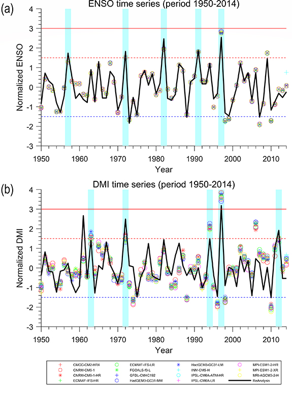
Figure 1. ENSO (a) and IOD (b) variability during the 1950–2014 period. Positive ENSO and IOD events (exceeding +1.5 standard deviation σ) are denoted by cyan shading. Red, dashed-red and dashed-blue lines indicate values of +3σ, +1.5σ and − 1.5σ, respectively. 1997 IOD event is considered an extreme positive event (exceeding +3σ). ENSO: El Niño–Southern Oscillation; IOD: Indian Ocean Dipole.
Download figure:
Standard image High-resolution imageWe noted that the spread between the models in simulating DMI was larger than the ENSO index, suggesting that the simulation of IOD events might still require improvement. Uncertainties exist in the trends of the frequency and strength of IOD events since the 1950s (Cai et al 2013), and these trends are dependent on specific SST data sets (Han et al 2014). Climate models exhibited biases in simulating the IOD (e.g. Weller and Cai 2013, Chu et al 2014) and ENSO (e.g. Taschetto et al 2014), and many of the well-known biases, such as the overly strong IOD amplitude, persist in CMIP6 models (McKenna et al 2020). However, the results of the present study indicate that data from the CMIP6 high-resolution models were useful in investigating the causal connections between ENSO and IOD.
3.1. Effects of ENSO on IOD during 1950–2014
The probability of no Granger causality from ENSO to IOD for the years 1950–2014 is presented in figure 2. Specifically, we only found the impact of ENSO at year t [i.e. D(t)JF(t + 1)] on the IOD at year t + 1 [i.e. SON(t + 1)], while ENSO at year t does not have predictive power on the IOD at year t + 2 [i.e. SON(t + 2)] and further years. The results of two models (INM-CM5-H and MPI-ESM1-2-XR) indicated that ENSO was considered unlikely to have no causal impact on the IOD, i.e. p-values were less than 0.33 (Stocker et al 2013). Most of the other models and reanalysis data had p-values of 0.33–0.66, suggesting that ENSO is as likely as not to have causal effects on IOD. A previous study (Le and Bae 2019), which used a different set of models (i.e. CMIP5 models with different model responses to greenhouse forcing), showed more likely significant ENSO influence on the tropical Indian Ocean and IOD during the years 2006–2100. Hence, the results of the present study suggested that the causal effects of ENSO on the IOD might be weaker during the years 1950–2014 compared to those in the future (2006–2100) when the greenhouse forcing is stronger. Moreover, the results supported the conclusions of previous studies (Saji et al 1999, Luo et al 2008, Izumo et al 2010, Le and Bae 2019, Abram et al 2020) regarding the possible independence of IOD variations from ENSO forcing. Other studies (e.g. Dong and Mcphaden 2017) have demonstrated recent changes in the relationship between the Pacific and Indian Oceans, and several IOD events occurred independently of ENSO conditions in the tropical Pacific. For example, two consecutive positive IOD events occurred in 2006 and 2007, together with a weak El Niño and La Niña, respectively (Luo et al 2008). Thus, the increased independence of the tropical Indian Ocean from the tropical Pacific Ocean forcing during the years 1950–2014 might not be uncertain.
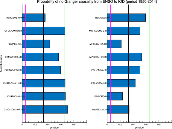
Figure 2. Probability for the absence of Granger causal effects from the ENSO to the IOD of 15 individual models and reanalysis data for the 1950–2014 period. ISMR and the SAM are the confounding factors (see Methods section 2.2). Green, black and magenta lines denote probability of 0.66, 0.33 and 0.05, respectively. ENSO: El Niño–Southern Oscillation; IOD: Indian Ocean Dipole; ISMR: Indian summer monsoon rainfall; SAM: Southern Annular Mode.
Download figure:
Standard image High-resolution imageFigure 3 details the response of tropical Indian Ocean SST (figures 3(a) and (b)) and surface zonal winds (figures 3(c) and (d)) during the boreal fall of year t + 1 [i.e. SON(t + 1)] to ENSO of year t [i.e. D(t)JF(t + 1)]. The model means (figure 3(a)) revealed the effects of ENSO on SST in parts of the southeastern tropical Indian Ocean, whereas according to the reanalysis data, ENSO impacted the southwestern tropical Indian Ocean close to Madagascar (figure 3(b)). ENSO may modulate surface zonal winds in the area of western Sumatra–Java (figures 3(c) and (d)) and parts of the northern tropical Indian Ocean (figure 3(d)). However, we found that the ENSO signature on the tropical Indian Ocean climate during the years 1950–2014 was weak in most regions, particularly the western tropical Indian Ocean.

Figure 3. ENSO [D(t)JF(t + 1)] effects on the boreal fall [SON(t + 1)] tropical Indian Ocean SST (a), (b) and surface zonal winds (c), (d). Red and green contour lines denote p-value = 0.05 and 0.1, respectively. Brown shades imply low probability for the absence of Granger causality. Stippling indicates that more than 70% of models agree on the multi-model mean probability. For a given model, the agreement is defined when the discrepancy between that model's probability and the multi-model mean probability is less than one standard deviation of the multi-model mean probability. ENSO: El Niño–Southern Oscillation; SST: sea surface temperature. DJF: December–January–February; SON: September–October–November.
Download figure:
Standard image High-resolution imageFurthermore, we noted that ENSO teleconnection to the western tropical Indian Ocean made an important contribution to ENSO's effects on the development of IOD (Le and Bae 2019). The weak control of ENSO in the western tropical Indian Ocean during the years 1950–2014 indicated the important role of internal Indian Ocean variability, which intensified under the warming environment. It is noted that the warming trend in the Indian Ocean since the 1950s is steeper than that in the tropical Atlantic and Pacific Oceans (Levitus et al 2009, Xue et al 2012). Moreover, the IOD interannual variability during this period mainly originated from internal changes in the Indian Ocean. These internal processes of the Indian Ocean are associated with both oceanic instabilities and stochastic atmospheric forcing (Han et al 2014). As the long-term warming trend in the western tropical Indian Ocean since the 1950s (Roxy et al 2014) was partly caused by the greenhouse effect (Hegerl et al 2007, Gleckler 2012, Park et al 2017), the weakened effects of ENSO on IOD might be due to increasing concentrations of anthropogenic greenhouse gases during the years 1950–2014.
Further analyses indicated that nonsignificant ENSO teleconnections to the tropical Indian Ocean are the results of weak ENSO modulation of Indo-Pacific Walker circulation (figure S1). Consistent with figures 3(c), (d) and S1 suggests that Indo-Pacific Walker cells simulated by the models do not extend to the western tropical Indian Ocean, which caused the nonsignificant effects of ENSO on these areas. The evolution of tropical Indian Ocean SST was significantly affected by ENSO during spring (figure S2), whereas these effects were reduced during summer (figure S3), demonstrating the seasonal cycle of tropical Indian Ocean SST. Importantly, the multi-model means (figures S2(a) and S3(a)) agreed with the reanalysis data (figures S2(b) and S3(b)) in terms of the effects of ENSO on western tropical Indian Ocean SST during the boreal spring and summer. These results suggest high agreement between the models and reanalysis data in reproducing the effects of ENSO on the tropical Indian Ocean.
3.2. Effects of IOD on ENSO during 1950–2014
Figure 4 describes the probability of no Granger causality from the IOD to ENSO during the years 1950–2014. As shown in equation 1 (Text S1), the effects of the IOD on ENSO are estimated on an annual basis (i.e. the IOD effects on ENSO of the following years are computed). All models had p-values of less than 0.33, indicating that the IOD was unlikely to have no causal impacts on ENSO during this period. The reanalysis data and simulations of three models (CMCC-CM2-HR4, FGOALS-f3-L and MPI-ESM1-2-HR, highlighted in yellow bars in figure 4) showed significant causal effects of IOD on ENSO at the 5% significance level. The 5% significance level was computed from the test for the null hypothesis of no Granger causality. We rejected this null hypothesis if the p-values were lower than 0.05, and we thus concluded that the causal effects were significant. Five models, CNRM-CM6-1, GFDL-CM4C192, INM-CM5-H, IPSL-CM6A-LR and MPI-ESM1-2-XR, exhibited significant causal effects of IOD on ENSO at the 10% significance level. These results demonstrated a robust causal influence of IOD on ENSO during the years 1950–2014.
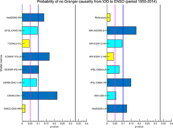
Figure 4. Probability for the absence of Granger causal effects from the IOD to ENSO of 15 individual models and reanalysis data for the 1950–2014 period. ISMR and the SAM are the confounding factors (see Methods section 2.2). Black, blue and magenta lines denote probability of 0.33, 0.1 and 0.05, respectively. Models having p-value < 0.05 are denoted by yellow bars, and models having 0.05 < p-value < 0.1 are denoted by cyan bars. ENSO: El Niño–Southern Oscillation; IOD: Indian Ocean Dipole; ISMR: Indian summer monsoon rainfall; SAM: Southern Annular Mode.
Download figure:
Standard image High-resolution imageThe responses of winter tropical Pacific SST and surface zonal winds of year t + 1 [i.e. D(t + 1)JF(t + 2)] to the IOD of year t [i.e. SON(t)] are depicted in figure 5. As expected, the multi-model results (figure 5(a)) and reanalysis data (figure 5(b)) indicated that the IOD had a strong signature over large parts of the tropical Pacific, particularly over the central-eastern areas. In addition, IOD impacts on southwestern tropical Pacific SST were observed. IOD signatures on surface zonal winds were observed in parts of the central and eastern tropical Pacific (figures 5(c) and (d)). These results agreed with previous studies that suggested that Indian Ocean warming enhanced Pacific trade winds and may induce changes in the Pacific climate (Luo et al 2012), and a positive IOD might cool the SST in the central Pacific (Izumo et al 2016) and eastern Pacific (Wang 2019) and play a part in the rapid phase transition from El Niño to La Niña (Yoo et al 2020). Other studies showed that Indian Ocean basin-wide warming (cooling) contributes to rapid termination of El Niño (La Niña) by inducing zonal wind anomalies over the equatorial western Pacific (Kug and Kang 2006, Izumo et al 2016) and suggested the strong interactions between the Pacific and Indian Oceans (Cai et al 2019). We observed high consistency between the models (highlighted as stippling in figure 5) in simulating the effects of the IOD on the tropical Pacific surface climate. Interestingly, the models and reanalysis data showed remarkable coherence in terms of the IOD signature on tropical Pacific surface climate. These results suggest the important role of the IOD in improving the predictability of tropical Pacific SST and surface zonal winds.

Figure 5. As in figure 3, but for IOD [SON(t)] effects on the boreal winter [D(t + 1)JF(t + 2)] tropical Pacific SST (a), (b) and surface zonal winds (c), (d). IOD: Indian Ocean Dipole; SST: sea surface temperature. DJF: December–January–February; SON: September–October–November.
Download figure:
Standard image High-resolution image
Further analyses revealed that the links between the IOD and tropical Pacific climate were associated with the modulation of Walker circulation connecting the tropical Indian Ocean and tropical Pacific (figure S4), where heat is transferred between these regions. As shown in figure S4 of the model mean results, the IOD [i.e. SON(t)] was likely to have causal effects on winter [i.e. D(t + 1)JF(t + 2)] 850 hPa zonal winds in central and parts of the eastern tropical Pacific, consistent with figures 5(a) and (c). These effects contributed to the influence of the IOD on the tropical Pacific climate described in figure 5. The IOD also induced deep atmospheric convection and caused a change in winter 250 hPa zonal winds (figure S5), implying a strong signature of the tropical Indian Ocean on different atmospheric levels of the tropical Pacific during the years 1950–2014. The IOD impacts were also tied to the SST anomalies in large parts of the tropical Pacific during the boreal summer (figure S6) and fall (figure S7), demonstrating the significant impact of the IOD on the development phase of ENSO. Interestingly, the patterns of IOD effects on the summer and fall SST were somewhat similar between the model means and reanalysis data (figures S6 and S7). These results indicated the capability of the models to reproduce the effects of IOD on the tropical Pacific. In addition, the results were consistent between high- and low-resolution models, suggesting that resolution might not significantly influence the representation of ENSO and IOD in the models (figure 1) or the interactions between these two modes (figures 2 and 4).
The interactions between ENSO and the IOD are expected to vary on long timescales (e.g. Santoso et al 2012, Ham et al 2017). The changes of the ENSO-IOD relationship can be observed in the sliding probabilities for the absence of Granger causality between ENSO and the IOD on a 41-year moving window (figure S8). The moving causal effects of ENSO on the IOD (figure S8(a)) are unstable during 1950–2014 in the models and reanalysis data. In reanalysis data, the p-values of the 1983–1991 central years show high fluctuation, suggesting possible decrease in ENSO effects during the 1963–2011 period. On the other hand, the moving causal effects of the IOD on ENSO are more significant (figure S8(b)) with most of the p-values being lower than 0.05 for the models' mean and reanalysis data. These results suggest more robust causal effects of the IOD on ENSO, consistent with the results described in figures 2 and 4.
4. Summary and conclusion
In this study, we examined the causal connections between IOD and ENSO during the years 1950–2014 using reanalysis data and simulations from CMIP6 high-resolution models. This period was of particular interest as rapid Indian Ocean warming since the 1950s has had significant impacts across the world (e.g. Roxy et al 2015). We revealed a more significant signature of IOD on ENSO interannual variability than vice versa during the years 1950–2014. All models demonstrated that IOD is unlikely to have no causal influences on ENSO (figure 4) during this period (p-values < 0.33), whereas eight of the 15 studied models and reanalysis data showed significant causal effects at the 10% significance level (p-values < 0.1). The links between the IOD and tropical Pacific climate were associated with the modulation of Walker circulation connecting the tropical Indian Ocean and tropical Pacific (figure S4), where heat is transferred between these regions. These impacts enhance the responses of winter tropical Pacific SST and surface zonal winds to IOD (figure 5). In addition, the IOD impacts were also tied to the SST anomalies in large parts of the tropical Pacific during the boreal summer (figure S6) and fall (figure S7), demonstrating the significant impact of the IOD on the development phase of ENSO. Most models (13 of 15) and reanalysis data (figure 2) indicated that ENSO was as likely as not to have causal effects on the IOD (p-values of 0.33–0.66). Non-significant ENSO effects on IOD were due to weakened ENSO influences on the western tropical Indian Ocean. This result was confirmed by both the reanalysis data and CMIP6 high-resolution models. The results demonstrated the overall independence of the IOD from ENSO forcing during the years 1950–2014, suggesting that the IOD interannual variability may have resulted primarily from internal Indian Ocean processes. Our analyses provide new evidence that ENSO interannual variability has likely been forced by changes in the IOD since 1950, indicating the necessity of considering Indian Ocean forcing to improve ENSO predictability. The increased impacts of the IOD were robust even for the short study period of 65 years as ENSO became a forced mode during the years 1950–2014 under global warming. Thus, the effects of the IOD on ENSO and the tropical Pacific might be more significant than previously thought. Given the projected increase in variability of the eastern Pacific El Niño (Cai et al 2018) due to greenhouse warming, we may expect stronger impacts of eastern Pacific El Niño on the IOD in the future. In addition, climate models projected an increase in frequency of extreme positive IOD and extreme El Nino events (Cai et al 2014a, 2014b). Hence, further studies related to the causal interactions between eastern Pacific ENSO and the IOD are necessary.
Acknowledgments
The authors thank the anonymous reviewers for their valuable comments and suggestions. We acknowledge the World Climate Research Programme, which through its Working Group on Coupled Modelling, coordinated and promoted CMIP6. We thank the climate modeling groups (listed in table S1) for producing and making available their model output, the Earth System Grid Federation (ESGF) for archiving the data and providing access, and the multiple funding agencies who support CMIP6 and ESGF. The 20th Century Reanalysis V2c data were provided by the NOAA/OAR/ESRL PSD, Boulder, Colorado, USA, from their website at www.esrl.noaa.gov/psd/. Kyung-Ja Ha was supported by the National Research Foundation of Korea (NRF) grant funded by the Korea government (MSIT) (Grant No. 2020R1A2C2006860).
Data availability statement
CMIP data can be downloaded from the ESGF website at https://esgf-node.llnl.gov/search/cmip6/. The 20th Century Reanalysis V2c data were provided by the NOAA/OAR/ESRL PSD, Boulder, Colorado, USA.