

Abstract
Mountain regions are experiencing more pronounced climate change than other global land areas. How have vegetation dynamics responded to these changes and what are the implications for hydrology? To answer these questions, we examine the impacts of changes in mean air temperature (Tmean), precipitation (P) and winter snow cover extent (SCE) in the headwaters of the Yellow River basin (HYRB) on two important vegetation dynamic metrics: (i) the maximum growing-season greenness (represented by the monthly maximum NDVI); and (ii) the beginning of growing season (BGS). Satellite-derived NDVI and SCE, along with observation-based gridded climate data, show that during the past 34 years (1982–2015) the HYRB experienced widespread vegetation greening, while no significant trend in BGS was observed. Spring greenness and phenology were significantly affected by SCE change, highlighting the importance of snow-related process to spring vegetation activity. We observed a clear signal of elevation-dependent warming below 4300 m elevation, which is absent at higher elevations. Changes in NDVI and BGS are elevation-dependent, and trends inTmean, P, and SCE with elevation play different roles in this dependence. Both observed and estimated watershed annual evapotranspiration series show increasing trends, suggesting that vegetation greening imposes positive effects on evaporative fluxes. Given steady-state and non-stationary hydrological conditions, increasing evapotranspiration should result in runoff reduction, which agrees with catchment-scale runoff observations across the HYRB. These findings represent new knowledge regarding the vegetation response to climate change in alpine environments which has important implications for the hydrology of the region and for other high-water yielding mountainous regions worldwide.
Export citation and abstract BibTeX RIS

Original content from this work may be used under the terms of the Creative Commons Attribution 4.0 license. Any further distribution of this work must maintain attribution to the author(s) and the title of the work, journal citation and DOI.
1. Introduction
Continuous climate warming over the last 50–100 years has imposed substantial stress on terrestrial ecosystem functioning, including vegetation phenology and productivity, distribution and composition of ecological communities, and has even shifted the range of some species (Beniston 2003, Diaz and Eischeid 2007). Both recorded and projected temperature changes suggest that mountainous regions are experiencing more substantial warming compared to other areas (Beniston 2003, Rangwala and Miller 2012). This has implications for energy and water balances, water resources and ecosystem adaption (Bradley et al 2004, Nogués-Bravo et al 2007, Mountain Research Initiative (MRI) EDW Working Group 2015). Wang et al (2014) analyzed the global 50-year trend of annual mean air temperature from 2367 stations and observed an enhanced warming rate of +0.19 °C per km for eight mountainous regions (including the Tibetan Plateau (TP), the western U.S., and the European Alps). Specifically, the warming rate of the northern TP was much greater than for the North China Plain (located at similar latitudes) being +2.1 and +1.5 °C per 50 years, respectively. Given this background, examining the response of montane ecosystems to warming is critical due to the important water resources they provide to both mountain communities and lowland residents (Viviroli et al 2011, Rangwala and Miller 2012, Minder et al 2018).
In a warming climate the hydrological cycle is intensifying (Huntington 2006). This implies that less winter precipitation will fall as snow, winter snowpacks will melt earlier in spring, and evapotranspiration will increase, with all else will being equal (Barnett et al 2005, Sorg et al 2012, Berghuijs et al 2014, Frans et al 2018, Mote et al 2018, Xu et al 2018). Montane ecosystems in arid and semi-arid regions are sensitive to spatial and temporal variability of hydrologic variables, especially variability in precipitation and snowpack (Stewart 2009). Precipitation provides available water for vegetation growth and plays a crucial role in arid and semi-arid ecosystem productivity (Liu et al 2016a). Snowpack can affect vegetation activity in numerous ways by regulating soil water and thermal processes (Maurer and Bowling 2014). These processes include microbial activity (Brooks et al 1996), root water and nitrogen uptake (Groffman et al 1999, Molotch et al 2009), vegetation leaf area and phenology (Trujillo et al 2012). While many investigations have explored the effects of climate change on alpine vegetation dynamics, most have focused on the influence of temperature change (table S1 (available online at stacks.iop.org/ERL/15/094005/mmedia)); the roles of precipitation and snowpack changes are yet not well understood and this paper fills that knowledge gap.
A number of recent studies analyzed elevation-dependent warming (EDW) and generally demonstrated that it has increased in recent decades (see (MRI 2015) and (Rangwala and Miller 2012) for comprehensive reviews of this topic, and table S1 for relevant studies and their key conclusions). Over the TP some studies reported EDW, yet other TP studies did not show EDW (table S1); so there is no strong consensus. For instance, Gao et al (2018) recently reported a clear EDW signal for the TP below 5000 m, while it was absent above this elevation. Given these conflicting results, further studies are required to explore whether, where, and to what extent changes in air temperature depend on the elevation. We found that vegetation greening over the northeastern TP was mediated by elevation in a previous study (Xu et al 2018). In the current work, analysis of changes in vegetation activity is taken one step further: to elucidate the seasonal difference of greening and changes in spring phenology with elevation and to explore the possible causes. These are critically important to understand ecosystem response to climate change in Alpine environment.
Here, we address three questions related to vegetation change over the headwaters of the Yellow River basin (HYRB) that is associated with general warming over the last three and a half decades. They are: (i) how has climate change impacted alpine vegetation dynamics? (ii) how have changes in air temperature varied with elevation, and how have vegetation dynamics responded to changes in air temperature? and (iii) how has vegetation change affected hydrologic processes?
2. Data and methods
Our study domain is the HYRB (∼122 000 km2; figure 1) which is located in the north-east of the TP, and experiences distinct wet and dry seasons in summer and winter, respectively. It is the 'water tower' of the much larger Yellow River basin (YRB) which is the home to an estimated 400 million people and has experienced dramatic climate change over the past four decades. Land cover is dominated by alpine grasslands including alpine steppe and alpine meadows (figure S1). The HYRB covers only 15% of the area of the entire YRB, but contributes approximately 35% of the total annual YRB discharge (Hu et al 2011).
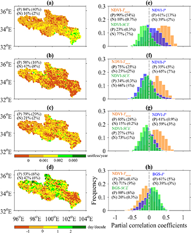
Figure 1. Spatial patterns of the 34-year (1982–2015) trends in NDVI during (a) spring, (b) summer, and (c) autumn, and of the trends in (d) the beginning of growing season (BGS) for the HYRB. Parts (e)–(g) show frequency distributions of partial correlation coefficients between corresponding seasonal NDVI and climate factors (mean air temperature (Tmean ), precipitation (P) and winter snow cover extent (SCE)), while (d) shows the frequency distribution between the BGS and spring Tmean , spring P and SCE. Parts (a)–(c) use the same color bar. Percentage of positive (P) and negative (N) trends and percentage of positive and negative correlations are provided (p < 0.05, percentage of significant trends/correlations in parentheses).
Download figure:
Standard image High-resolution image2.1. Data
Our study period is from 1982 to 2015. The data we used include: (i) the long-term AVHRR (Advanced Very High Resolution Radiometer) GIMMS3 g (Global Inventory, Monitoring, and Modelling Studies) NDVI product (GIMMS3 g thereafter; Tucker et al 2005); (ii) the MODIS NDVI product (MOD13C2, Collection 6, Didan et al 2015); (iii) the observation-based gridded climate data (mean air temperature (Tmean ), precipitation (P) and downward longwave radiation (Rld )) (He et al 2011); (iv) the snow cover extent (SCE) product of Hori et al (2017); (v) the GLEAM (Global Land-surface Evaporation Model) evapotranspiration product (Miralles et al 2011); (vi) the SRTM 1 km DEM data (http://srtm.csi.cgiar.org/); and (vii) the hydrologic data (runoff and pan evaporation (E0 )). Table 1 summarizes the period of observations, spatiotemporal resolution, and data source for each data set. More detailed descriptions are provided in the supplementary material.
Table 1. Summary of the data sets used in this study.
| Data | Temporal extent | Temporal resolution | Spatial resolution | Data source |
|---|---|---|---|---|
| GIMMS3 g NDVI | 1982–2015 | Biweekly | 1/12 degree | https://ecocast.arc.nasa.gov/data/pub/gimms/3g.v1/ |
| MODIS NDVI | 2000–2015 | Monthly | 0.05 degree | https://lpdaac.usgs.gov/products/mod13c1v006/ |
| Observed spring phenology | 2003–2011 | — | — | Zhang et al 2013 |
| Climate data | 1982–2015 | Monthly | 0.1 degree | http://westdc.westgis.accn/data/ |
| Snow cover extent | 1982–2015 | Biweekly | 0.05 degree | http://kuroshio.eorc.jaxa.jp/JASMES/ |
| GLEAM evapotranspiration | 1982–2015 | Daily | 0.25 degree | https://www.gleam.eu/ |
| DEM | — | — | 1 km | http://srtm.csi.cgiar.org/ |
| Runoff | 1982–2015 | Daily | — | Ministry of Water Resources of China |
| Pan evaporation | 1982–2015 | Daily | — | http://data.cma.cn/ |
2.2. Methods
2.2.1. Evaluating spatiotemporal consistency between GIMMS3 g and MODIS NDVI datasets
We removed contamination in the NDVI signal related to clouds and snow following Fensholt and Proud (2012) which is based on pixel-level QA information in the original biweekly GIMMS3 g NDVI products (see supplementary material). To further reduce the influence of clouds and snow and match the temporal resolution of MODIS-based NDVI product, we aggregated the biweekly data to monthly using the maximum value compositing approach (Fensholt and Proud 2012). NDVI exhibits some scale dependency because the index is a non-linear transformation (Fensholt and Proud 2012) and therefore we did not perform spatial resampling of the MODIS 0.05-degree data directly on the NDVI data. Rather, we resampled the MOD13C2 red and near-infrared reflectance data to match the GIMMS3 g 1/12-degree spatial resolution by spatial averaging, and then recalculated NDVI from the reflectance data. Areas with low NDVI values (<0.1 annual mean) are excluded since those areas indicate sparse vegetative or bare soil areas (Zhou et al 2001). There are 1713 1/12-degree spatial resolution pixels covering the HYRB. We calculated the per-pixel Pearson correlation coefficient (r) from overlapping 16-year monthly observations as the strength of the linear association between GIMMS3 g and MODIS monthly NDVI as a basis for assessing the quality of the GIMMS3 g NDVI data. We estimated trends in growing-season (defined as 1 March through 30 November) NDVI average using linear least squares regression to produce per-pixel maps of r and slope values to evaluate the consistency between the two data sets. Typically, r ranged from 0.73 to 0.98 with high values occurring in the southeastern HYRB with high NDVI and low values in a small part of the northwest HYRB with low NDVI (figure S2(a)). Trend analysis result shows that spatial patterns of the two data sets were consistent (figures S2(b)–(c)). Overall, the performance of the GIMMS3 g NDVI product was acceptable for detecting long-term trends in vegetation dynamics over the study domain (supplementary text); similar to Beck et al's (2011) finding globally. We noted that slopes of MODIS NDVI trends were slightly higher compared to that of GIMMS3 g archive (figure S2(d)), which suggested that the magnitude of the vegetation change over the longer 34-year period is probably underestimated.
2.2.2. Impact of climate change on montane vegetation dynamics
We examined two important vegetation dynamic metrics: (i) the maximum growing-season greenness (represented by the monthly maximum NDVI); and (ii) the beginning of growing season (BGS). Due to the sparse ground observations, assessment of BGS changes on the HYRB is heavily dependent on remote sensing data. The cloud- and snow-removed biweekly GIMMS3 g NDVI data were used to retrieve BGS. We used a six-degree polynomial function (equation (1)) to reconstruct daily NDVI time series (Piao et al 2006). Then, following White et al (2009), we employed a dynamic local threshold NDVI ratio of 0.5 based on the annual minimum and maximum values to determine the beginning of growing season (BGS) for each pixel (equation (2)).


where t is the day of year (DOY), parameters a1, a2, ..., an are the fitted coefficients (using least squares). NDVIratio(t) is the estimated ratio of NDVI change which varies from 0 to 1.0; NDVImin and NDVImax are the annual minimum and maximum NDVI.
Although the biweekly composited GIMMS3 g NDVI product is widely used to detect vegetation phenology at both regional and global scales (e.g. White et al 2009, Julien and Sobrino 2009, Jeong et al 2011), there is still a debate regarding the sufficient temporal resolution for retrieving vegetation phenology. For example, Zhang et al (2009) evaluated the impacts of compositing period on vegetation phenology detection based on the 16 d MODIS Enhanced Vegetation Index (EVI) data. They found that time series with a temporal resolution of 6–16 d were sufficient for accurate detection of several phenology events. Pouliot et al (2011) compared satellite-derived spring green-up onset date with in situ observations for deciduous forests and found that compositing periods ranging from 7 to 11 d provided the best estimates for leaf out. Coarser or finer compositing periods resulted in a greater error. Comparing the estimated BGS with in situ observations during 2003–2011, we found that the mean estimated BGS was DOY 142 ± 8 and the mean BGS estimated from eight agro-meteorological stations (dominated by alpine grassland) was DOY 136 ± 10. Due to the biweekly temporal resolution of the NDVI, such errors are expected. We note that the temporal sensitivity for accurately detecting vegetation phenology from satellite-based vegetation data is still poorly understood. We strongly suggest that much effort be directed towards comparing satellite-based vegetation phenology from multiple temporal resolutions with field observations in the future.
Some studies have found that vegetation responds differently to daytime (Tmax ) and nighttime (Tmin ) warming in the temperate steppe of northern China (Shen et al 2016, Xu et al 2018), eastern Europe, southern Siberia, western America (Xia et al 2014, Tan et al 2015), and eastern Canada (Rossi and Isabel 2017). Our results indicate that the inter-annual variations in growing season NDVI were more strongly associated with changes in Tmax than those in Tmin in the HYRB (figure S3). We estimated the sensitivity of NDVI to Tmax (or Tmean ) based on multiple linear regressions with NDVI as the dependent variable and Tmax (or Tmean ), P and SCE as independent variables. We found that the mean sensitivity of NDVI to Tmean was slightly higher compared to that of Tmax (figure S4). Therefore, we did not consider the non-uniform (daytime/nighttime) warming because this effect is smaller than changes in Tmean . We used the Mann-Kendall (MK) test (two-tailed test) to determine whether pixel-level and basin-scale temporal trends in vegetation greenness (monthly maximum NDVI), BGS and climate factors were statistically significant (p < 0.05). Positive and negative trends indicate greening and browning in NDVI (or delaying and advancing in BGS), respectively. The magnitude of the trend was determined using linear regression. We evaluated the strength of relationships between the two vegetation metrics (greenness and BGS) and climate factors using partial correlation analysis (Liu et al 2016a). This method can explore correlations between NDVI/BGS and single climate variable while removing effects of the two remaining climate variables in this study. We defined spring as March through May, summer as June through August, autumn as September through November, and winter as December through the next February.
2.2.3. Pattern of air temperature change with elevation and response of vegetation dynamics
Important information can be lost and potential errors introduced if slope variations within a given elevation band are not accounted for (Fang and Huang 2004), because the frequency distribution of elevation is non-uniform. Here, we regarded variations in temporal trends in Tmean (ΔTmean ) with elevation as well as other climatic factors and vegetation metrics as a one-dimensional signal, and applied wavelet transforms to remove the noise (extreme value for a given elevation range) using the symlet 5 (sym5) wavelet decomposition. The symlet family is useful for denoising, as they have no explicit mathematical expressions and only can be solved numerically (Daubechies 1992). Following denoising, we examined trends in selected variables for possible elevation dependencies. Previous studies have found that mechanisms closely related to EDW include snow-albedo feedbacks and water vapor changes (Rangwala and Miller 2012, MRI 2015). We identified ΔSCE, ΔP and ΔRld as possible causes for elevation gradients in ΔTmean . To investigate their relative contributions to EDW, we first examined patterns of possible drivers with elevation to ensure the selected factors exhibited clear elevation dependence, and then we performed a correlation analysis and stepwise regression to identify the primary driver of ΔTmean .
2.2.4. Hydrological implications of vegetation dynamic change
As vegetation dynamics are strongly coupled with the latent heat flux (Schlesinger and Jasechko 2014), temporal trends in annual actual evapotranspiration (ETa ) will be consistent with those in annual integrated NDVI and BGS. That is, increases in NDVI and/or earlier BGS should lead to increases in ETa , and vice versa. As reliable estimation of long-term ETa remains a challenging problem in hydrologic research (Lettenmaier et al 2015, Purdy et al 2018), we estimate ETa using multiple methods to reduce uncertainties. Because transpiration and canopy interception are positively related to leaf area index (LAI) and soil evaporation is negatively related to LAI, their contribution to ETa changes should be different. To evaluate this, we investigated temporal trends in ETa and its components. In addition to ETa calculated from water-balance and by GLEAM, we also estimated sequential 5-year averages of ETa using the generalized Budyko equation (equation (3)) (Choudhury 1999). This equation assumes that changes in water storage can be ignored at long-term annual scale (Roderick and Farquhar 2011).
where n is a catchment-specific parameter, which modifies the partitioning of P between ETa and runoff. We used a recommended default value of n = 1.8 (Choudhury 1999). E0 is catchment-averaged pan evaporation.
3. Results and discussion
3.1. Impact of climate change on montane vegetation dynamics
During the 34-year period (1982–2015), trends in NDVI were positive for 84%, 58% and 79% of the HYRB pixels in spring, summer and autumn, respectively; with 40%, 16% and 29% being statistically significant (p < 0.05; see figures 1(a)–(c)). The relative contribution of pixels with negative trends to total pixels was 16%, 42%, and 21% in spring, summer and autumn, respectively. The corresponding seasonal percentages with significant negative trends was 2%, 8% and 19%, respectively. Regional inter-annual NDVI in spring showed significant increasing trends at a rate of 0.006 per year (not statistically significant in summer and autumn) (figures 2(a)–(c)). Pinzon and Tucker (2014) analyzed uncertainties or errors of the GIMMS3 g NDVI data and found that errors resulted from seasonal variations, which contributed the largest proportion of the total error, depend upon NDVI values. That is, large errors correspond to high NDVI values. They estimated a total error of ±0.005 NDVI units. Due to relatively small NDVI values in the HYRB (figures 2(a)–(c)), minor uncertainties are expected. However, one should use the NDVI data with caution for climate change research.
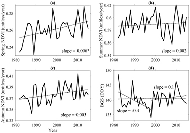
Figure 2. Inter-annual variations of HYRB-averaged NDVI during three seasons (a)–(c) and (d) the beginning of growing season (BGS) over 1982–2015. Slopes marked with star mean that the trend is significant (p < 0.05).
Download figure:
Standard image High-resolution imageWe examined linkages between vegetation growth and climate factors and found that NDVI was positively correlated with Tmean during the three non-winter seasons (figures 1(e)–(g)). There were positive partial correlations in 90%, 75% and 85% of the HYRB in spring, summer and autumn, respectively, with 54%, 25% and 28% of correlations being statistically significant. In spring, 61% of the pixels had positive partial correlations between vegetation greenness and P, while in summer and autumn, the partial correlations were negative in 65% and 59% of the pixels, respectively. Partial correlations between NDVI and SCE were dominantly negative in spring and ambiguous in summer and autumn. The results suggest that growing-season greening was primarily stimulated by climate warming across the HYRB. This finding is consistent with previous studies of the entire TP (Zhang et al 2013), the western U.S. (Cayan et al 2001), and central Europe (Kudernatsch et al 2008). We note that evidence from field warming experiments demonstrates that rising temperatures relax low-temperature limitations and enhance alpine grassland growth (Kudernatsch et al 2008, Wang et al 2011, 2012), which are consistent with our own.
We observed early BGS in the southeastern HYRB, whereas later BGS was mainly in the northwestern HYRB (figure S5(a)), which followed the spring gradient of temperature and precipitation. The growing season started in the middle of May in most areas while other areas exhibited earlier (beginning of April) or later (end of May) growing season (figure S5(b)). BGS trend analysis revealed that 53% had positive trends, of which 6% were statistically significant (figure 1(d)). Regionally, we found no significant trends in BGS over the entire study period. However, we identified two distinctly different trends between 1982–1998 and 1998–2015. During 1982–1998, BGS significantly advanced by 4 d/decade which is similar to the mean advancing rate of growing season in North America (4 d/decade) and Eurasia (3 d/decade) (Zhou et al 2001). In contrast, BGS had a small delay of 1 d/decade during 1982–1998 (figure 2(d)). Inter-annual variations in spring temperature show that the HYRB exhibited continuous warming between 1982 and 2015 (figure S6(a)) which allows us to suggest a non-linear response of spring phenology to temperature change. Climate warming has been widely recognized as advancing spring vegetation phenology, while both in situ observations and satellite records reveal that warming in autumn and winter decreases the fulfilment of chilling requirements and result in later spring green-up onset (Zhang et al 2007, Guo et al 2015). This was supported by weaker correlations between BGS and spring temperature during 1998–2015 than the period of 1982–1998 (figure S7).
We found negative partial correlations between BGS and spring Tmean at 71% of pixels; 9% of correlations were statistically significant (figure 1(h)). Partial correlations between BGS and spring P were generally positive. Our results indicate that both spring warming and wetting could promote advancing of spring phenology. This is mainly because higher temperature and precipitation in spring enhances photosynthesis and alleviates water stress. In addition to temperature and precipitation, BGS may also have been affected by reduced winter snow cover. Partial correlations between BGS and SCE were positive for 80% of the area, with 6% of the correlations being statistically significant. This finding highlights the important role of snow-related processes in alpine grassland spring vegetation activity.
3.2. Patterns of temperature change with elevation and vegetation dynamics response
We observed enhanced warming at elevations below 4300 m, but warming rates greatly declined above this elevation (figure 3(a)). Examining patterns of possible causes with elevation, we found spring P increased with elevation, while summer and autumn P shifted from negative trends to positive trends at about 4000 m and increased at higher elevations (figure 3(b)). SCE declined at lower elevations but increased above 4650 m (figure 3(c)). Generally, Rld increased at each elevation which could be attributed to increased water vapor (figure 3(d)). The pattern of ΔRld with elevation was very similar to that of ΔTmean . A correlation analysis showed that ΔTmean was statistically significant and positively related to ΔRld but negatively related to ΔP and ΔSCE. We used a stepwise regression model to investigate their combined effects and to identify the primary driver of ΔTmean . Inclusion of the three independent variables (i.e. ΔRld , ΔP and ΔSCE) accounted for 83%, 91%, 83% and 90% variance of ΔTmean during spring, summer, autumn and the growing season, respectively (table 2). Among the three variables, ΔRld played a leading role followed by ΔSCE and ΔP, as the ΔRld univariate model explained most of the variance of ΔTmean (table 2). It should be noted that the gridded precipitation data were developed using more than one dataset as background (including station observations, TRMM satellite precipitation, and GLDAS precipitation data) which would introduce uncertainties and biases in the data time series (Beck et al 2020).
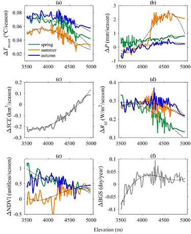
Figure 3. Changes in the 1982–2015 trends as a function of elevation of (a) mean air temperature (ΔTmean ; °C/season), (b) precipitation (ΔP; mm/season), (c) winter snow cover extent (ΔSCE; km2/season), (d) downward longwave radiation (ΔRld ; W/m2/season), (e) NDVI (ΔNDVI; unitless/season), and (f) the beginning of growing season (ΔBGS; day/year) over the HYRB. A third-order polynomial was used to examine the general pattern of each variable, the equations are provided in supplementary material table S2.
Download figure:
Standard image High-resolution imageTable 2. Determination coefficient (R2 ) of the seasonal univariate, bivariate and trivariate stepwise regression models in which temporal trends in mean air temperature (ΔTmean ) is the dependent variable and temporal trends in downward longwave radiation (ΔRld ), winter snow cover extent (ΔSCE) and precipitation (ΔP) are independent variables.
| Univariate model | Bivariate model | Trivariate model | |||||||
|---|---|---|---|---|---|---|---|---|---|
| ΔRld | ΔSCE | ΔP | ΔRld & ΔSCE | ΔRld & ΔP | ΔP & ΔSCE | ΔRld , ΔSCE & ΔP | |||
| Spring | 0.82 | 0.52 | 0.55 | 0.83 | 0.85 | 0.64 | 0.85 | ||
| Summer | 0.75 | 0.37 | 0.38 | 0.85 | 0.88 | 0.41 | 0.88 | ||
| Autumn | 0.37 | 0.30 | 0.32 | 0.61 | 0.65 | 0.35 | 0.67 | ||
| Growing season | 0.83 | 0.43 | 0.48 | 0.85 | 0.86 | 0.50 | 0.86 | ||
Most studies reported enhanced warming at higher elevations (table S1; Nogués-Bravo et al 2007, MRI 2015), however, we observed EDW only below 4300 m. Our results are generally consistent with Gao et al (2018) who analyzed changes in temperature with elevation over the TP using observed, reanalyzed and WRF (Weather Research and Forecasting) model simulated data. They found a clear signal of EDW below 5000 m, but reported that neither ERA-Interim reanalysis nor the WRF model indicated EDW above this elevation. They explored the physical process based on WRF output and found that snowpack showed an increasing melt under 5000 m resulting in lower albedo. However, increased snowfall in a warmer climate partially compensates for increased snowmelt and thus leads to a little change in albedo above 5000 m. Gao et al (2018) further concluded that EDW above 5000 m elevation over the TP is unlikely to occur in future decades based on their analysis of WRF climate projections. Our findings support their conclusion although with a somewhat different elevation threshold. As there is no strong consensus on EDW even within the same region, future studies should aim to accurately detect the signal and mechanisms through combined analysis of observations, model-simulated and satellite-retrieved datasets.
Examining changes in the two vegetation metrics with elevation, we found that spring and autumn ΔNDVI corresponded well with the concurrent pattern of ΔTmean (figure 3(g)), suggesting a strong control of the elevation gradient of ΔTmean on vegetation greening in two seasons. Summer NDVI exhibited browning trends below 4000 m and increased greening trends above this elevation. Because this pattern was consistent with the elevation gradient of summer ΔP, it can be reasonably inferred that ΔP was likely an important regulator of summer vegetation greenness across the elevation range. This result suggests a high sensitivity of vegetation growth to summer precipitation in semi-arid environments (Poulter et al 2013). Carlson et al (2017) investigated changes in peak NDVI (NDVImax) with elevation in the Ecrins National Park (within the French Alps) and found that the highest proportional increases in NDVImax occurred in the rocky habitats at high elevation. They attributed possible causes to glacier retreat, decrease in snow cover duration, and increased atmospheric nitrogen deposition at high elevations. Noting that they calculate relative values of NDVImax trends rather than absolute values which is likely to change the elevation-dependence patterns, we analyzed relative values of NDVI trends with elevation as well. The result shows that the general patterns of the relative change in NDVI with elevation were consistent with absolute values (figure S8). Therefore, the elevation-dependent response of greening is closely related to patterns of local climate change. ΔBGS showed an evident elevation gradient with greater rates of advance occurring at lower elevations (figure 3(h)), which are positively related to ΔSCE and spring ΔTmean .
Other studies have also observed elevation dependence of changes in greenness and BGS (e.g. Piao et al 2011, Li et al 2015), but most attributed the cause to EDW. Our findings reveal that seasonal changes in ΔTmean, P, and SCE with elevation played different roles in the vegetation dynamic response. This is the first time that the impacts of P and SCE changes with elevation on vegetation activity have been evaluated in the region. The aspect is another important topographic factor that promotes variations in energy and water in complex terrain (Fan et al 2019). We analyzed changes in growing season NDVI and BGS with aspect and found that vegetation greening was slightly higher on the south, southwest and west slopes, while there were no obvious differences in spring and autumn (figures S9(a)–(c)). BGS advanced on the southeast and northwest slopes and delayed at other slopes (figure S9(d)). The elevation dependency of the vegetation dynamic changes has important implications for energy and mass balance of the high-mountain regions and associated hydrology and also for species that live in narrow habitats (MRI 2015). We assume that climate change is the main controller of elevation dependency of vegetation dynamics. Our analysis may overstate the influence of climate on vegetation growth if non-climatic factors that vary with elevation help explain spatial pattern of vegetation dynamics.
Another problem that mountain regions face globally is the lack of observations at high elevations. Taking the elevational distribution of precipitation observations as an example, the GPCC (Global Precipitation Climatology Centre) archive shows that precipitation observations for elevations above 2500 m are under-represented (above this elevation only 0.2% of the 48 767 GPCC precipitation stations are located (excluding Greenland and Antarctica)). In terms of network density per continent, Asia has the lowest density (0.02 stations per 100 km2 or 5633 km2 per station) and the value above 2500 m is even lower (0.004 stations per 100 km2 or 26 692 km2 per station) (Viviroli et al 2011). Environmental monitoring stations (at which both hydrometeorological and ecological observations are made) should be installed at higher-elevation and ecologically sensitive locations which exhibit rapid and detectable changes, rather than being located (as at present) in lower elevations, notwithstanding a range of pragmatic challenges associated with higher elevations, experiencing more extreme conditions and affordability.
3.3. Hydrological implication of vegetation dynamic change
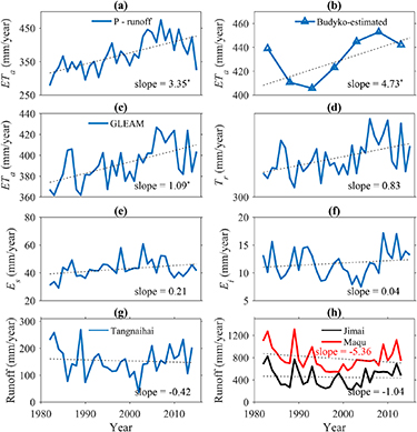
Annual HYRB-averaged ETa calculated from water balance (P − runoff) varied between 278.3 and 475.1 mm/year with a mean value of 371.0 mm/year during 1982–2015. The Budyko-estimated ETa ranged from 405.7 to 452.8 mm/year with a mean value of 431.1 mm/year. The GLEAM ETa rates exhibited smaller temporal variability during 1982–2015 with a mean value of 391.9 mm/year (figures 4(a)–(c)). The considerable discrepancy between the measured and GLEAM-estimated ETa series is possibly due to its great underestimation of potential evaporation in comparison with pan evaporation (figure S10). With differences in magnitude among ETa time series neglected, all three showed significant positive trends during the past 34 years, suggesting that vegetation greening and/or earlier growing season are imposing positive effects on evapotranspiration. This agrees with both global and regional analyses that vegetation greening and growing-season advancing are important drivers of long-term ETa variations (Ukkola et al 2016, Zhang et al 2016, Liu et al 2016b). For example, Zeng et al (2018) quantified the potential effect of the satellite-observed global greening on the terrestrial hydrologic circle by using a coupled land-climate model and found that 8% increase in LAI resulted in 55% ± 25% increase in observed ETa during 1982–2011.
Figure 4. Inter-annual variations of actual evapotranspiration (ETa ), ETa components and runoff. Parts (a)–(c) display ETa calculated from the water balance equation, the generalized Budyko equation, and from the GLEAM product. Parts (d)–(f) show inter-annual variations of GLEAM transpiration (Tr ), soil evaporation (Es ) and canopy interception (Ei ), respectively. Parts (g) and (h) show inter-annual variation of runoff from three hydrological stations located within the HYRB. The Tangnaihai station samples the entire HYRB, whereas the Jimai and Maqu stations are located in the upper and middle HYRB, respectively (figure S2(c)). Slopes marked with star mean the trend is significant (p < 0.05).
Download figure:
Standard image High-resolution image
We also examined temporal variations of the ETa components from GLEAM products, the results of which showed that annual transpiration and canopy interception increased by 0.83 and 0.04 mm/year whereas soil evaporation increased by 0.21 mm/year, which further supports our assumption (figures 4(d)–(f)). Because reliable estimation of long-term ETa and its components remains a challenging problem in hydrologic research (Lettenmaier et al 2015, Purdy et al 2018), comprehensive intercomparison within and between output of land surface models and satellite-derived ETa products provides robust support for our assumption which could motivate future research. Analyzing runoff variation in the study domain, we found that annual runoff from three hydrological stations in the upper, middle and lower HYRB (see figure S2(c) for specific location of each station) all showed decreasing trends with different magnitudes (figures 4(g)–(h)). Zhang et al (2018) recently reported that, in arid and semi-arid China (which includes the HYRB), increased LAI has resulted in an 8.5% runoff reduction in 1990 s and 11.7% reduction in 2000 s compared to the 1980 s baseline. Our findings along with the abovementioned study provide evidence at catchment/regional scale for potential drying environment and reducing water resource.
Our analysis is a first step in establishing the variation of ETa and runoff as related to vegetation change in the study domain. Hydrologic models assume that vegetation dynamics (vegetation greenness, types, phenology and density) are static, whereas both our findings and those of other research show that elevation dependence of vegetation greenness and phenology changes is likely (Piao et al 2011, Trujillo et al 2012, Li et al 2015). Goulden and Bales (2014) found that both eddy covariance measurements and remotely sensed annual ETa (calculated from MODIS NDVI data) in California's upper Kings River basin peaks at mid-elevation (about 2000 m) and declines at lower elevation due to water availability limitation and upper elevation due to temperature limitations. They explored sensitivity of river flow to vegetation expansion and found that continuous warming is expected to expand ETa upslope due to vegetation redistribution and to increase basin ETa and decrease runoff. It is also important to elucidate the runoff sensitivity to vegetation change at different elevation bands to fully evaluate the impact of climate change on mountain hydrology of the HYRB. However, it is not possible at present due to the sparsely distributed weather and hydrologic observations in the harsh environment.
4. Conclusions
With respect to the three questions raised in the Introduction, we can make the following conclusions. Firstly, during the past 34 years, the HYRB experienced widespread vegetation greening and slightly delayed BGS. Spring greenness and phenology were significantly affected by SCE change, highlighting the importance of snow-related process in spring vegetation activity. Secondly, we observed a clear signal of EDW below 4300 m, whereas it was absent above this elevation. Spring and autumn greening corresponded well with the elevation gradient of warming, while summer greening appeared to be regulated by patterns of precipitation changes with elevation. Note that the precipitation change results should be treated with caution due to the sparse observations and uncertainties of the gridded precipitation in the HYRB. Changes in the BGS experienced evident elevation dependency with greater advancing rates occurring at lower elevations, which was closely related to the pattern of spring temperature and SCE changes. To our knowledge, it is the first time that the impacts of precipitation and SCE changes with elevation on vegetation activity are evaluated. Thirdly, both observed and estimated annual ETa time series showed increasing trends, suggesting that vegetation greening would impose positive effects on the latent heat flux. Given steady-state and non-stationary hydrological conditions, increasing ETa is expected to result in runoff reduction, which agrees with catchment-scale runoff observations across the HYRB.
Acknowledgments
This work was funded by the National Key R&D Program of China (Grant No. 2016YFC0402710); the National Natural Science Foundation of China (Grant No. 51539003); the Fundamental Research Funds for the Central Universities (Grant Nos. 2018B608X14; 2019B80214); and the Postgraduate Research & Practice Innovation Program of Jiangsu Province (Grant No. KYCX18_0580). We thank three anonymous referees for the detailed and constructive comments and Zhaojun Zheng for his helpful suggestions on the selection of snow cover products.
Data availability statement
Any data that support the findings of this study are included within the article.