

Abstract
The exchange of carbon between the Earth's atmosphere and biosphere influences the atmospheric abundances of carbon dioxide (CO2) and methane (CH4). Airborne eddy covariance (EC) can quantify surface-atmosphere exchange from landscape-to-regional scales, offering a unique perspective on carbon cycle dynamics. We use extensive airborne measurements to quantify fluxes of sensible heat, latent heat, CO2, and CH4 across multiple ecosystems in the Mid-Atlantic region during September 2016 and May 2017. In conjunction with footprint analysis and land cover information, we use the airborne dataset to explore the effects of landscape heterogeneity on measured fluxes. Our results demonstrate large variability in CO2 uptake over mixed agricultural and forested sites, with fluxes ranging from −3.4 ± 0.7 to −11.5 ± 1.6 μmol m−2 s−1 for croplands and −9.1 ± 1.5 to −22.7 ± 3.2 μmol m−2 s−1 for forests. We also report substantial CH4 emissions of 32.3 ± 17.0 to 76.1 ± 29.4 nmol m−2 s−1 from a brackish herbaceous wetland and 58.4 ± 12.0 to 181.2 ± 36.8 nmol m−2 s−1 from a freshwater forested wetland. Comparison of ecosystem-specific aircraft observations with measurements from EC flux towers along the flight path demonstrate that towers capture ∼30%–75% of the regional variability in ecosystem fluxes. Diel patterns measured at the tower sites suggest that peak, midday flux measurements from aircraft accurately predict net daily CO2 exchange. We discuss next steps in applying airborne observations to evaluate bottom-up flux models and improve understanding of the biophysical processes that drive carbon exchange from landscape-to-regional scales.
Export citation and abstract BibTeX RIS

Original content from this work may be used under the terms of the Creative Commons Attribution 4.0 licence. Any further distribution of this work must maintain attribution to the author(s) and the title of the work, journal citation and DOI.
1. Introduction
The terrestrial biosphere plays a dynamic role in the global carbon cycle, removing an estimated 25%–30% of the carbon dioxide (CO2) emitted from human activity (Ciais et al 2013, Le Quéré et al 2018). However, the prognosis for this sink remains poorly constrained due to uncertain climate feedbacks on the atmosphere-biosphere cycling of CO2 (Cox et al 2013, Wenzel et al 2016, Bond-Lamberty et al 2018). In addition, the land biosphere acts as a net source of methane (CH4) (Saunois et al 2016, Tian et al 2016), with large uncertainties (>20 Tg yr−1) in magnitudes and ecosystem-dependent responses to climate state (Turner et al 2019). Thus, it is critical to accurately determine CO2 and CH4 fluxes, and their associated sensible and latent heat fluxes, from landscape-to-regional scales to better constrain the global carbon budget.
Several approaches exist for quantifying terrestrial carbon exchange. Top-down methods use a combination of observed atmospheric mixing ratios, transport models, and prior emissions estimates to infer fluxes of CO2 (Houweling et al 2015, Wang et al 2018) and CH4 (Bousquet et al 2011) on regional to global scales. These atmospheric inversion models provide a useful constraint on flux but offer limited attribution information on the underlying biophysical factors driving the carbon cycle. Bottom-up methods, in contrast, rely on biomass inventories (e.g. Pacala et al 2001, Pan et al 2011), surface flux tower networks (Baldocchi et al 2001, Jung et al 2011), or biophysical process models (e.g. Schaefer et al 2008) to extrapolate flux from local to global scales. However, inventory-based estimates have large associated uncertainties of up to 75% (Hayes et al 2018), and discrepancies persist between different modeling approaches (Huntzinger et al 2012, Melton et al 2013) and model-tower data comparisons (Schwalm et al 2010, Schaefer et al 2012). Tower-based flux observations can provide benchmark information and a basis for validation, but their spatial representativeness is very limited at regional to continental scales (Villarreal et al 2018).
Airborne eddy covariance (EC) provides near-direct measurements of surface-atmosphere exchange over landscape-to-regional scales (e.g. Lenschow et al 1981, Desjardins et al 1982, 1989, Crawford et al 1996, Sellers et al 1997, Gioli et al 2004, Sayres et al 2017, Wolfe et al 2018). Such observations have successfully been used to evaluate CH4 emissions inventories (Hiller et al 2014) and to scale up tower- or aircraft-based fluxes via empirically-derived environmental response functions (Miglietta et al 2007, Metzger et al 2013, Zulueta et al 2013). Airborne EC has also been applied to validate regional-scale flux inversions (Lauvaux et al 2009), light-use efficiency models of carbon and energy fluxes (Kustas et al 2006, Anderson et al 2008), and biophysical process models of forest carbon exchange (Maselli et al 2010).
Attribution of airborne fluxes requires knowledge of the spatial contribution of surface fluxes to the measurement at aircraft altitude: the flux footprint (Leclerc and Thurtell 1990, Schuepp et al 1990). In conjunction with surface information (e.g. thematic land cover), footprint analysis enables the allocation of fluxes to the underlying surface state. For example, the flux fragment method decomposes fluxes using the subset of observations that have a homogeneous footprint in the EC calculation (Kirby et al 2008, Dobosy et al 2017, Sayres et al 2017). While this method is highly reliable, it is best suited to regions with sufficient homogeneity to capture enough single-footprint observations, or to aircraft flying low enough to minimize the footprint size. More complex algorithms incorporate footprint-weighted land cover information to decompose observed fluxes using numerical or regression analysis (Chen et al 1999, Ogunjemiyo et al 2003, Wang et al 2006, Hutjes et al 2010). Such methods are more practical for data sets with mixed underlying terrain.
Here, we utilize an extensive airborne flux dataset to explore the effects of surface heterogeneity on the land-atmospheric exchange of sensible and latent energy, CO2, and CH4. Footprint analysis in conjunction with thematic land classification maps demonstrates that airborne fluxes can resolve spatial heterogeneity in land type at the 1–2 km2 scale. We highlight campaign results for two case studies: a predominantly agricultural area between Maryland and Delaware, and a wetland forest located in coastal North Carolina. We further evaluate campaign measurements against flux observations from several towers and explore whether empirical time trends from towers yield a means of scaling airborne flux samples to net daily CO2 exchange. Finally, we discuss next steps in utilizing airborne observations to calibrate and evaluate modeled flux products.
2. Methods
2.1. Airborne flux campaign and data
The NASA Carbon Airborne Flux Experiment (CARAFE) platform, payload, and data processing are described in detail by Wolfe et al (2018). The data presented here were collected during two CARAFE deployments in September 2016 and May 2017. Flights spanned the Mid-Atlantic states and targeted a variety of land-use and ecosystem types, including forests, agricultural lands, and wetlands. Flux transects (figure 1) cumulatively comprise ∼7000 km of linear distance, with typical altitudes of 80–300 m. EC fluxes of sensible heat (H), latent heat (LE), CO2 (FCO2), and CH4 (FCH4) were determined via continuous wavelet transforms (Torrence and Compo 1998), as detailed in Wolfe et al (2018) and summarized in section S1.1, available online at stacks.iop.org/ERL/15/035008/mmedia. 1 Hz processed flux data from the CARAFE campaigns, in addition to supporting scalar and winds data, are publicly available: https://air.larc.nasa.gov/missions/carafe/index.html.

Figure 1. Map of the NASA CARAFE flux transects from September 2016 (red) and May 2017 (cyan). All flights were based out of Wallops Flight Facility (WFF) in Wallops, VA. The locations of five flux towers situated beneath the flight tracks are indicated by white triangles.
Download figure:
Standard image High-resolution image2.2. Flux tower data
CARAFE flights included ∼50 overpasses of flux towers (figure 1). Table 1 lists key information for each tower. The USDA Choptank (USDA-Chop) tower is situated in the Choptank River watershed, an agricultural area of predominantly soy and corn crops on the eastern shore of the Chesapeake Bay (Sun et al 2017). The remaining four towers are part of the larger AmeriFlux network. The St. Jones tower (US-StJ) samples the St. Jones Reserve tidal marsh in southeastern Delaware (Capooci et al 2019). The Cedar Bridge tower (US-Ced) and the Silas Little tower (US-Slt) are both located in the Pinelands National Reserve in southern New Jersey, with mostly pitch pine-dominated stands near US-Ced and mixed oak stands near US-Slt (Clark et al 2018). The US-NC4 tower is located in the Alligator River National Wildlife Refuge, a forested swamp in North Carolina (Miao et al 2017). Tower sites processed EC flux data according to standardized AmeriFlux procedures, as summarized in section S1.2, and AmeriFlux data are publicly available: https://ameriflux.lbl.gov. All towers report H, LE, and FCO2, while the US-StJ and US-NC4 locations additionally report FCH4. With the inclusion of a small storage correction (typically <10%), towers also report net ecosystem exchange (NEE). Note that NEE is opposite in sign to FCO2. The tower fetch across all sites ranges from 100 to 2500 m.
Table 1. Summary of flux towers underlying CARAFE flight tracks. The primary NLCD 2016 land class is also listed.
| Tower | Description | Lat, Long | Land class | Measurements | Overfly date |
|---|---|---|---|---|---|
| US-Ced | Cedar Bridge, NJ | 39.8379° N | Evergreen forest | H, LE, FCO2 | 20160914 |
| 74.3791° W | 20160923 | ||||
| 20170509 | |||||
| US-Slt | Silas Little, NJ | 39.9138° N | Deciduous forest | H, LE, FCO2 | 20160914 |
| 74.5960° W | 20160923 | ||||
| 20170509 | |||||
| US-NC4 | Alligator River, NC | 35.7879° N | Woody wetlands | H, LE, FCO2 | 20160924 |
| 75.9038° W | FCH4 | 20170515 | |||
| 20170526 | |||||
| US-StJ | St. Jones, DE | 39.0882° N | Herbaceous wetlands | H, LE, FCO2 | 20160912 |
| 75.4372° W | FCH4 | 20170504 | |||
| 20170518 | |||||
| USDA-Chop | Choptank, MD | 39.0587° N | Cultivated crops | H, LE, FCO2 | 20160912 |
| 75.8513° W | 20170504 | ||||
| 20170518 |
2.3. Flux decomposition by land class
2.3.1. Land classification
Land cover information was taken from the National Land Cover Database (NLCD 2016), a high-resolution (30 m × 30 m) map based on Landsat imagery (Yang et al 2018). The CARAFE domain includes 14 of the 20 NLCD land classes. Dominant land classifications sampled during CARAFE include woody wetlands (45%), cultivated crops (22%), and dry forests (evergreen, deciduous, and mixed classes) (21%). The remaining types are developed land (open, low, medium, and high density), open water, emergent herbaceous wetlands (hereafter herbaceous wetlands), shrubs, pastures, and grasslands, which individually make up less than 5% of the cumulative footprint.
2.3.2. 2D flux footprint analysis
The flux footprint relates the spatial distribution of fluxes at the surface ( ) to the observed flux (
 ) measured at coordinates
  and measurement height
  (Horst and Weil 1992, Schmid 1994):
where, x and y are arbitrary horizontal coordinates and f is the flux footprint function, which expresses the contribution of each upwind unit surface element to  We use the two-dimensional Flux Footprint Prediction (2D-FFP) developed by Kljun et al (2015), a parameterization based on a Lagrangian stochastic particle dispersion model (Kljun et al 2002) that is applicable to many turbulence regimes and measurement heights. The parameterization utilizes the following inputs: measurement height
  the mean horizontal wind speed U, the planetary boundary layer height
  the Obukhov length
  the standard deviation of the lateral (crosswind) velocity fluctuations
  and the friction velocity u*. We derive
  from the wavelet variances of the horizontal wind velocity vectors.
We calculate the 2D-FFP for all 1 Hz data points (∼75 m distance at typical flight speed) along all flux transects below 200 m. Each data point has an associated  but leg-average values of the micro-meteorological variables (i.e.
  ) are used as the FFP is based on a mean flow parameterization, and point-to-point momentum fluxes exhibit significant variability. We estimate the boundary layer height from vertical profiles before and after each set of flux transects as described in Wolfe et al (2018). Note that even a 20% error in
  has less than a 0.5% impact on the size and distribution of the footprint, except in highly stable conditions (Kljun et al 2015) atypical during the CARAFE flights. Once calculated, the 2D-FFP was rotated into the mean wind direction and transformed into the geographic coordinate space of the measurement, generating a gridded map of the footprint function associated with each flux observation. Figure 2 depicts an example of a single footprint for a flux measurement from the 18 May, 2017 flight to Choptank, MD superimposed on the NLCD 2016 land cover map. For all flux observations from the 2016 and 2017 campaigns below 200 m in altitude, the 90% upwind extent for calculated footprints ranged from 1.5 to 10 km.

Figure 2. A single flux transect from the 18 May, 2017 flight over the Choptank/St. Jones region, overlaid on the NLCD 2016 land cover map. The grey shading indicates the cumulative footprint for all observation points along the leg. The inset box shows a single 2D footprint calculated using the Kljun et al (2015) parameterization, with black contours depicting weighted contributions to the observed flux from 10% to 90% in 10% increments. The white arrow denotes the mean horizontal wind direction, and the magenta circle indicates the 200 m radius around the USDA-Choptank tower.
Download figure:
Standard image High-resolution image2.3.3. Disaggregation into component fluxes
To derive fluxes representative of a single land class, we use the Disaggregation combining Footprint analysis and Multivariate Regression (DFMR) methodology described by Hutjes et al (2010). DFMR relies on the flux footprint and land cover to estimate a weighted contribution of each land class to the flux measurement. The observed flux,  can be written as a linear summation of component fluxes from each of n land classes within the footprint:

where  is the fractional area of the kth land class within the footprint and
  is the corresponding component flux, or the mean land-class flux for a given set of observations (i.e. a single flight). The values
  can be determined using the flux footprint function f to weight the relative contributions of land cover patches within the footprint, as patches closer to the sensor influence the measurement more heavily than patches farther away (equations (S1) and (S2)).
The multiple linear regression (equation (S3)) was performed on a flight-by-flight basis to derive land-class component fluxes for each flight. A grid of 2D-FFP values was superimposed onto the NLCD 2016 map to generate the weighted fractional area of each land class in every footprint (see figure 2). Although NLCD displayed 14 land classes in our sampling region, we down-selected for land classes that constituted more than 20% of the footprint-weighted area in at least 4 km of cumulative (but not necessarily consecutive) flux observations. This screening criterion, which was optimized via comparison with flux sub-samples from homogeneous footprints (figure S1), ensured that selected land types were sampled enough to provide a meaningful average.
In addition to residual error, random and systematic measurement errors (see Wolfe et al 2018) were propagated through the regression, and errors were summed in quadrature to yield the total uncertainty for each component flux. Uncertainties in a priori surface characterization and footprint extent are not included. While the footprint calculation should introduce minimal error (barring significant changes to the fractional areas), mischaracterization of the surface cover could introduce significant biases. Corrections for vertical flux divergence are likewise not included due to large uncertainties in the correction factors (see Wolfe et al 2018). The flights all took place near midday and targeted fair-weather conditions. However, the data are not screened for the presence of clouds, and such variations may contribute another source of flux variability in addition to those discussed below.
3. Results and discussion
3.1. Disaggregated fluxes by region
3.1.1. Choptank watershed and St. Jones Reserve
CARAFE deployments included three flights to the Choptank agricultural area (12 September 2016, 4 May 2017, and 18 May 2017). Flux transects spanned the Delmarva peninsula from the Chesapeake Bay to the Atlantic Ocean (typical length 60 km) and included overflights of the USDA-Chop and US-StJ towers (figure 1). This region had mixed terrain, with six land classes meeting the down-selection criteria described in section 2.3.3. Table 2 summarizes footprint-weighted contributions of each land class.
Table 2. Summary of land cover contributions for the Choptank/St.Jones and Alligator River case studies. FP-weighted area is the mean for all flights to that region.
| Region | Land class | FP-area |
|---|---|---|
| Choptank/St. Jones | Cultivated crops | 56% |
| Woody wetlands | 21% | |
| Deciduous forest | 6% | |
| Developed-Open | 6% | |
| Herbaceous | <5% | |
| wetlands | <5% | |
| Open water | ||
| Alligator River | Woody wetlands | 83% |
| Open water | 10% | |
| Cultivated crops | <5% | |
| Herbaceous | <5% | |
| wetlands |
Disaggregated fluxes highlight the variability in carbon dynamics between land classes and over time (figure 3). Of particular interest, cultivated crops (e.g. annual crops such as soybean or corn) and forested lands (e.g. woody wetlands and deciduous forest) display substantial differences in FCO2 for the sampling periods. The CO2 uptake from cultivated crops ranged from −3.4 ± 0.7 to −11.5 ± 1.6 μmol m−2 s−1, whereas deciduous and wetland forests display a much larger uptake, ranging from −12.1 ± 3.9 to −22.7 ± 3.9 μmol m−2 s−1 and −9.1 ± 1.5 to −22.7 ± 3.2 μmol m−2 s−1, respectively. Forest uptake of CO2 also dominates that by croplands in other regions with substantial cropland fraction (figures S2, S3). While the difference in CO2 uptake between croplands and forest will be strongly dependent on crop type and phenology (Lokupitiya et al 2009), crops in the CARAFE region are typically in their early growth stages in May and undergoing senescence in September. Developed open lands, which comprise mostly lawn grasses and vegetation with <20% impervious surface area, also draw down substantial CO2 (∼−13 to −30 μmol m−2 s−1) during the May sampling period.

Figure 3. Disaggregated fluxes by land class for flights to the Choptank Watershed region: (a) sensible heat flux; (b) latent heat flux; (c) CO2 flux; and (d) CH4 flux. Land class fluxes are grouped by fractional area and ordered by flight date from left to right. Note that September dates are from the 2016 campaign and May dates are from 2017. Error bars represent ±2σ uncertainty in the component flux, which includes systematic and random error propagated through the regression analysis, in addition to the regression residuals. CARAFE was not sampling fast CH4 measurements on May-18, and no FCH4 data are available on this date.
Download figure:
Standard image High-resolution imageChoptank data also exhibit a general anticorrelation between FCO2 and LE, expected for vegetated land surfaces where transpiration and stomatal control is a major contributor to evapotranspiration. The sampling is too limited to infer much about seasonal flux response for the various land types, but forested lands are comparably photosynthetically active during the growing season between May and September.
The disaggregation methodology also illustrates FCH4 variability with land type. FCH4 observations were at or below the detection limit for most CARAFE flights, and uncertainties are large due to poorly constrained regression results. However, it is known that soils from forested ecosystems represent a weak CH4 sink (Subke et al 2018), whereas tree stems represent a weak CH4 source (Vargas and Barba 2019) that may counterbalance ecosystem scale CH4 fluxes in upland forested ecosystems. In contrast, herbaceous wetlands, located primarily on the Eastern end of the track near the St. Jones tower, exhibit relatively strong CH4 emissions of 76.1 ± 29.4 nmol m−2 s−1 on Sep-12 and 32.3 ± 17.0 nmol m−2 s−1 on May-04. This region has a mix of herbaceous wetlands that extend across a salinity gradient, where lower CH4 emissions may be associated with wetlands in brackish waters and larger CH4 emissions with freshwater wetlands (Poffenbarger et al 2011, Capooci et al 2019).
3.1.2. Alligator river
Three flights over the Alligator River region took place during the CARAFE deployments on 24 September 2016, 15 May 2017, and 26 May 2017. Flux transects spanned the Alligator River National Wildlife Refuge in the N–S direction, with the US-NC4 tower located near the middle of the flight transects (see figure 1). The dominant land cover contributions included woody wetlands, open water, and some minor areas of cultivated crops and herbaceous wetlands. Table 2 contains a summary of the land-cover contributions to the footprint for Alligator River region.
The component fluxes from Alligator River display significant variability with land type (figure 4). For example, the open water component of H is at or near zero for all flights, and evaporation dominates the surface energy fluxes for this class, as displayed by LE values generally greater than 200 W m−2. Note that although classified as open water in the NLCD, the coastal waters sampled near Choptank and Alligator River are actually comprised of estuarine waters and tidal mudflats. We observed occasional CO2 emissions from these waters of 6.2 ± 2.2 μmol m−2 s−1 over the Alligator River (Sep-24, figure 4) and 6.4 ± 3.7 μmol m−2 s−1 in the Choptank region (May-18, figure 3). Both regions also display positive fluxes of CH4, with means of 40.5 ± 12.2 nmol m−2 s−1 over the Alligator River and 20.5 ± 10.1 nmol m−2 s−1 in Choptank. These values are within the range of prior flux estimates, which can be up to ∼10 μmol CO2 m−2 s−1 in low salinity estuarine waters, and ∼30–35 nmol CH4 m−2 s−1 in tidal mudflats (Abril and Borges 2005).
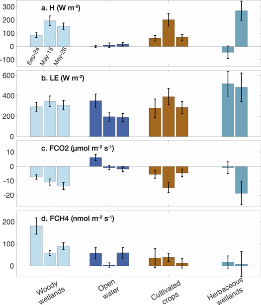
Figure 4. As in figure 3, but for flights to the Alligator River in North Carolina. Emergent wetlands were not sufficiently represented in the Sep-24 observation footprints.
Download figure:
Standard image High-resolution imageThe woody wetlands land class, a freshwater forested swamp in the Alligator River region, also displays persistent, large CH4 emissions ranging from 58.4 ± 12.0 to 181.2 ± 36.8 nmol m−2 s−1. These remarkably high values are recurrent and consistent over long periods at this site (Mitra et al 2019a), which has recorded among the highest CH4 emissions from wetlands globally, including tropical wetlands. Other temperate swamplands exhibit mean CH4 emissions of ∼35 nmol m−2 s−1 (Turetsky et al 2014), but few global observational records exist for wetland ecosystems.
3.2. Comparison to tower flux observations
Direct comparison of aircraft and tower flux observations is challenging in heterogeneous landscapes, as the two platforms often sample different terrain due to the mismatch in footprint size (on the order of ∼100 m for towers and ∼3 km for CARAFE flights). During the CARAFE campaign, most flights contained numerous land cover types within a single footprint (figure 2), resulting in an amalgamated signal from land-use and ecosystem states with varied carbon fluxes. In contrast, each tower sampled the local surface state with footprints that were typically homogeneous.
For each flight, tower data are averaged over the duration of the flight and compared to the aircraft disaggregated component flux corresponding to the tower's primary land class (figure 5). Note that the aircraft component flux is derived using data from the entire flight region, and thus we are comparing a mean regional land-class flux to the site-specific land-class flux at the tower location. The correlation between aircraft and tower fluxes varies between species, with H exhibiting the strongest correlation (r2 = 0.76, figure 5(a)) and the tightest fit (NRMSE = 15%). The slope of 0.58 ± 0.21 indicates a low bias in the aircraft fluxes, which may stem from the vertical flux divergence, which has not been included in the disaggregation. Divergence corrections typically range from ∼10% to 60% with uncertainties of greater than 30% in the correction factors. LE fluxes display a slightly weaker correlation (r2 = 0.53, figure 5(c)) with notably more scatter between the aircraft and tower observations (NRMSE = 30%). FCO2 demonstrates similar scatter between the aircraft component fluxes and tower observations (NRMSE = 30%) but shows a weaker overall correlation (r2 = 0.30) that may be skewed by a couple of outlying points in the US-Slt comparison (figure 5(b)). The slopes for both LE (0.74 ± 0.31) and FCO2 (0.68 ± 0.31) contain substantial uncertainty in magnitude. The limited number of tower FCH4 observations make quantitative comparison with the aircraft fluxes difficult, and the correlation is not statistically significant, with a p-value > 0.05 (figure 5(d)). Nonetheless, aircraft data overrepresent CH4 fluxes at US-StJ and underrepresent CH4 fluxes at US-NC4.

Figure 5. Comparison of disaggregated aircraft fluxes and tower fluxes by land class for (a) sensible heat, (b) CO2, (c) latent heat, and (d) CH4. Error bars for aircraft observations indicate ±2σ uncertainty, which includes systematic and random error propagated through the regression analysis, in addition to the regression residuals. Tower errors are assumed to be ± 10%. The dashed line is the 1:1 reference, and the solid grey line indicates the best fit, with slope and intercept reported with 95% confidence intervals. The towers sample the following land classes: evergreen forest (US-CED), deciduous forest (US-Slt), cultivated crops (USDA-Chop), woody wetlands (US-NC4), and herbaceous wetlands (US-StJ).
Download figure:
Standard image High-resolution imageComparisons between the aircraft and tower observations suggest that local tower measurements capture 30%–76% of the variance in regional ecosystem-dependent fluxes. The larger scatter (and weaker correlation) in observations of LE and FCO2 as compared to H could in part stem from errors in source area attribution. For example Kustas et al (2006) and Bertoldi et al (2013) found that footprint extents can differ between active (e.g. T) and passive scalars (e.g. H2O, CO2) in heterogeneous landscapes. A full quantification of the source contribution error requires computationally expensive boundary layer flow simulations outside the scope of this study.
Despite potential footprint inconsistencies, variability in the underlying drivers of carbon exchange within a land type expectedly results in discrepancies between aircraft and tower observations. In the Choptank watershed, where cultivated crops dominate the footprint, the disaggregation could be further refined based on crop type or land-use inventories to better quantify the effect of these parameters on CO2 uptake (e.g. Zhang et al 2015). Additionally, forested classes dominate several regions in the CARAFE domain, including the Alligator River and Pocomoke Forest (table S2). Combining land cover with maps of forest canopy structure (Hurtt et al 2004) or metrics of photosynthetic activity, such as solar-induced fluorescence or vegetation indices (Frankenberg et al 2011), could provide additional observational constraints on the regional heterogeneity in the CO2 sink.
In wetland regions, the underlying biogeochemical factors that control CH4 emissions are not implicit with land class, and in some circumstances, CH4 fluxes can be highly episodic and localized (Whalen 2005). For example, CH4 fluxes in the brackish herbaceous wetlands near the US-StJ site depend on flooding and drying conditions that change salinity gradients across the tidal zone (Capooci et al 2019). In the freshwater forested wetlands near US-NC4, Mitra et al (2019b) found that methanogen substrate availability produced via photosynthesis largely controls CH4 flux, whereas water-table depth and surface temperature played a non-causal role in emissions. The complexity of the underlying controls of CH4 fluxes stresses the need for continued regional-scale studies of these important yet understudied wetland ecosystems.
Although the observed variability in flux cannot be fully attributed to land class, the results emphasize the utility of spatially distributed observations in probing carbon cycle dynamics across heterogeneous regions. Typically, flux tower networks are used as ground-truth observations to evaluate carbon exchange in process models (Friend et al 2007, Raczka et al 2013) and to inform a priori errors in atmospheric inversions (Chevallier et al 2006). However, individual tower sites are limited in regional representativeness (this work, Villarreal et al 2018), and aircraft EC can provide a valuable supplement with which to examine landscape-scale changes in the underlying drivers of carbon exchange.
3.3. Upscaling with tower temporal trends
Tower flux observations offer a long-term record of local carbon cycle dynamics, of which aircraft observations only capture a brief subsample. Here, we explore whether the temporal record of NEE from towers can inform the extrapolation of local fluxes to regional, daily-integrated values using aircraft observations.
The tower sites included in the CARAFE domain demonstrate a distinct correlation between daily- and peak-NEE for the 2016 annual datasets (figure S5). We define peak-NEE as the mean CO2 exchange between 11:00 and 15:00 local, the time of day in which maximum CO2 uptake by the biosphere is usually observed. Most CARAFE flights took place within this time frame. Daily-NEE is the 24 h integral of half-hourly or hourly tower measurements. Figure 6(a) depicts the linear least squares fits of daily- versus peak-NEE for each individual tower site colored by land class, and the fit parameters and uncertainties are summarized table 3. Note that this analysis does not account for inter-annual variability.

Figure 6. Linear fits of the daily—NEE versus peak—NEE for the five tower sites in 2016 (a). The fits are colored by the tower land class: US-Ced (deciduous forest), US-Slt (mixed forest), US-NC4 (woody wetland), USDA-Chop (cultivated crops), US-StJ (herbaceous wetlands). Monthly mean diurnal CO2 fluxes for US-Ced and US-StJ during August 2016 (b). The shaded area indicates the ±1σ of all NEE observations over the given timeframe.
Download figure:
Standard image High-resolution image
Table 3. Linear regression parameters for daily NEE versus peak-NEE both in units of μmol m−2 s−1 calculated using the flux tower observations from 2016. Slope and intercept are listed with 95% confidence intervals.
| Tower | Slope | Intercept | r2 | RMSEa |
|---|---|---|---|---|
| US-Ced | 0.31 ± 0.02 | −0.64 ± 0.16 | 0.78 | 0.90 |
| US-Slt | 0.30 ± 0.02 | −0.84 ± 0.15 | 0.81 | 1.04 |
| US-NC4 | 0.30 ± 0.02 | −0.44 ± 0.11 | 0.83 | 0.73 |
| US-StJ | 0.21 ± 0.02 | −1.10 ± 0.30 | 0.54 | 1.95 |
| USDA-Chop | 0.27 ± 0.01 | −0.36 ± 0.12 | 0.88 | 0.89 |
Four of the five tower sites display similar relationships between peak and daily exchange, with a mean slope of 0.30 ± 0.02, excluding US-StJ. The St. Jones tower samples a variable footprint, creating more scatter in the daily- versus peak-NEE (see figure S5, table 3), and this site is strongly influenced by tides, which are known to affect diel patterns of NEE (Kathilankal et al 2008). Furthermore, mean diurnal NEE profiles for the month of August 2016 shown in figure 6(b) reveal a larger ecosystem respiration from this land class as compared to other tower sites, accounting for the shallower slope of 0.21 ± 0.02. Nonetheless, the generally high correlations suggest that peak-NEE is predictive of net daily exchange across land types in the CARAFE domain, and peak CO2 fluxes observed during the midday CARAFE flights encapsulate 50%–90% of the day-to-day variability in carbon exchange. The temporal relationships observed at the tower sites thus provide a mechanism for inferring regional daily carbon exchange via airborne sampling.
Despite the similar relationships between daily- and peak-NEE across tower sites, ecosystem-dependent variability still results in large differences in carbon exchange, within and across individual days (e.g. figures 3 and 4). A full assessment of the relationships between peak-NEE and longer-term trends is beyond the scope of this work. However, Zscheischler et al (2016) have shown that observations of annual NEE from several tower sites in temperate forests, including US-Ced and US-Slt, demonstrate a strong correlation with the number of days having ecosystem fluxes above a high percentile. These analyses indicate that such temporal relationships can provide an empirical proxy for the climatic factors driving longer-term variability in carbon exchange. Furthermore, extracting longer-term information from airborne fluxes can facilitate comparison with flux inversions and process models, which often lack fine-timescale resolution.
4. Conclusions
We demonstrate that airborne fluxes, when combined with footprint and land cover information, resolve spatial heterogeneity in landscape flux. During the September and May sampling periods, results often show substantial differences in FCO2 with land type, and forests typically display a larger CO2 uptake than croplands. This likely stems from the fact that in May most crops are typically still in early development and by September they are undergoing senescence heading towards harvest, whereas forests are consistently photosynthetically active during this time frame. We also observe a small but significant source of CH4 from estuarine waters and tidal mudflats. Larger CH4 emissions of up to ∼75 nmol m−2 s−1 are observed near the St. Jones Reserve, a brackish herbaceous wetland, and up to ∼180 nmol m−2 s−1 in the Alligator River Refuge, a freshwater woody wetland.
Our results also suggest that the tower sites located along the flight path capture ∼30%–75% of the regional variability in ecosystem-dependent fluxes of H, LE, and FCO2, but the limited number of tower sites with FCH4 observations makes quantitative comparison difficult. Diversity in the underlying biophysical drivers of flux within land classes likely accounts for the observed regional-scale ecosystem variability. Moreover, the underlying biogeochemical controls of CH4 flux in wetlands are often not directly tied to land class, including such factors as substrate availability, salinity, and water table depth. The persistently high CH4 emissions observed during CARAFE at the local US-StJ and US-NC4 tower sites emphasize the need to further test the representativeness of these understudied and heterogeneous ecosystems.
Although towers offer limited regional representativeness both within and across ecosystem states, tower observations complement airborne EC by providing a long-term record of ecosystem-dependent carbon cycling. The tower sites in the CARAFE domain display nearly consistent relationships between peak- and daily-CO2 exchange (within uncertainty), suggesting a means of upscaling to regional daily carbon cycle dynamics via airborne measurements.
While this study focused on thematic land cover, a wealth of remote sensing data yields unique opportunities to assess model-derived fluxes and quantify uncertainties in regional flux products. Potential future work includes extending the disaggregation methodology to derive relationships between observed fluxes and surface parameters such as canopy height, solar-induced chlorophyll fluorescence, or normalized difference vegetation index that initialize model- and satellite-derived fluxes (e.g. Hurtt et al 2004, Zhang et al 2014), thus enabling direct evaluation. Additionally, the spatially-distributed fluxes from airborne EC provide the unique capability of evaluating landscape-scale flux maps derived from remote sensing models (Anderson et al 2008) as well as gaining a greater understanding of boundary layer dynamics affecting flux footprint and source area modeling using large eddy simulations (Bertoldi et al 2013).
The importance of terrestrial ecosystems in the global CO2 and CH4 budgets motivates the need for continued measurements over regions where large uncertainties in carbon exchange persist, such as natural wetlands and areas of rapid environmental and land-use change. Incorporating remote-sensing surface information could further focus such studies, exploiting the full potential of airborne flux observations in constraining carbon cycle dynamics.
Acknowledgments
The CARAFE 2016 and 2017 missions were supported by the GSFC Internal Research and Development Program, the NASA Carbon Monitoring System Program (NNH15ZDA001N-CMS), and the NASA HQ Earth Science Division. We also acknowledge the following AmeriFlux sites for their data records: US-Ced, US-NC4, US-Slt, and US-StJ. Funding for the AmeriFlux data resources was provided by the US Department of Energy's Office of Science, and additional support for the US-StJ tower came from NSF grant #1652594. Research and flux data from US-Ced and US-Slt were supported by the Northern Research Station, USDA Forest Service. Data from the USDA-Agricultural Research Service is part of the Long-Term Agroecosystem Research (LTAR) program.
Data availability
The data that support the findings of this study are openly available at the following DOIs: 10.17190/AMF/1480314; 10.17190/AMF/1246096; 10.17190/AMF/1246043; 10.17190/AMF/1480316. All data are available upon request from the corresponding author, and aircraft data can be publicly accessed: https://air.larc.nasa.gov/missions/carafe/index.html.