

Abstract
Since the mid-1800s pinyon-juniper (PJ) woodlands have been encroaching into sagebrush-steppe shrublands and grasslands such that they now comprise 40% of the total forest and woodland area of the Intermountain West of the United States. More recently, PJ ecosystems in select areas have experienced dramatic reductions in area and biomass due to extreme drought, wildfire, and management. Due to the vast area of PJ ecosystems, tracking these changes in woodland tree cover is essential for understanding their consequences for carbon accounting efforts, as well as ecosystem structure and functioning. Here we present a carbon monitoring, reporting, and verification (MRV) system for characterizing total aboveground biomass stocks and flux of PJ ecosystems across the Great Basin. This is achieved through a two-stage remote sensing approach by first using spatial wavelet analysis to rapidly sample tree cover from very high-resolution imagery (1 m), and then training a Random Forest model which maps tree cover across the region from 2000 to 2016 using temporally-segmented Landsat spectral indices obtained from the LandTrendr algorithm in Google Earth Engine. Estimates of cover were validated against field data from the SageSTEP project (R2 = 0.67, RMSE = 10% cover). Biomass estimated from cover-based allometry was higher than estimates from the Forest Inventory and Analysis Program (FIA) at the plot-level (bias = 5 Mg ha−1 and RMSE = 15.5 Mg ha−1) due in part to differences in tree-level biomass allometrics. County-level aggregation of biomass closely matched estimates from the FIA (R2 = 0.97) after correcting for bias at the plot level. Even after many previous decades of encroachment, we find forest area (i.e. areas with ≥10% cover) increasing at a steady rate of 0.46% per year, but 80% of the 9.86 Tg increase in biomass is attributable to infilling of existing forest. This suggests that the known consequences of encroachment such as reduced water availability, impacts to biodiversity, and risk of severe wildfire may have been increasing across the region in recent years despite the actions of sagebrush steppe restoration initiatives.
Export citation and abstract BibTeX RIS

Original content from this work may be used under the terms of the Creative Commons Attribution 4.0 licence. Any further distribution of this work must maintain attribution to the author(s) and the title of the work, journal citation and DOI.
1. Introduction
Dryland biomes cover 41.5% of the terrestrial earth surface and support 1079 million hectares of forest land (Bastin et al 2017). Rapid encroachment of woody plants into grasslands and savannas across the world (Stevens et al 2017) suggests that dryland regions are capable of supporting even greater amounts of woody biomass. Tracking the changes in woody cover and biomass of these systems is essential for understanding their role in the global carbon cycle and the numerous impacts of woody encroachment including changes to biodiversity (Miller et al 2000, Ratajczak et al 2012), ecohydrology (Huxman et al 2005, Roundy et al 2014, Kormos et al 2017), and ecosystem services (Anadón et al 2014, Kim et al 2016).
In particular, pinyon-juniper (PJ) and western juniper forests and woodlands of the western US (hereafter referred to as PJ woodlands) have received much attention due to their extensive encroachment since the mid-1800s which has displaced sagebrush steppe shrublands and grasslands and associated wildlife (Miller et al 2000, Romme et al 2009, Baruch-Mordo et al 2013). PJ ecosystems now cover over 40 million hectares (Romme et al 2009), making them the third largest vegetation type in the United States (Huang et al 2009). Although the density of carbon stored in these ecosystems is relatively low compared to other forest types, the vast area of short stature forests and woodlands (both nationally and globally) make them critical components of regional, national, and global carbon budgets. Furthermore, the carbon balance of these systems is extremely dynamic as evidenced by historic patterns of woody encroachment as well as recent large-scale mortality events in PJ ecosystems across the Intermountain West and southwestern US (Scholes and Archer 1997, Breshears et al 2005, Strand et al 2008, Clifford et al 2011). In addition to natural mortality, PJ ecosystems are actively managed to restore historic grassland and shrubland ecosystems, mainly for enhancing forage for livestock grazing and improving wildlife habitat quality for certain species such as the greater sage-grouse (Centrocercus urophasianus) (Miller and Rose 1999, Miller et al 2008, Romme et al 2009). Indeed, these natural and human induced changes have significant impacts on total carbon stocks and fluxes in PJ ecosystems, ultimately impacting carbon budgets at the national scale.
Despite their importance, carbon stocks and dynamics in PJ ecosystems are poorly quantified, and thus not well understood. This is partly due to the relative paucity of systematically collected field observations. Although the USDA Forest Service Forest Inventory and Analysis (FIA) program has plots in PJ woodlands, many areas do not meet the definition of forestland and thus are not included in the inventory or subsequent carbon reports such as the Environmental Protection Agency's annual emissions report (EPA 2019). Remote sensing can augment field observations to better quantify carbon stocks and fluxes in these ecosystems. However, most previous research using remote sensing to map PJ cover or biomass has either been limited to landscape scales or only one or two points in time (Smith et al 2008, Strand et al 2008, Falkowski et al 2017). Recently, remote sensing aided mapping of all carbon pools in the Great Basin of the western United States, including PJ, found nearly twice the total carbon of previous estimates which were limited to forest areas (Fusco et al 2019). These methods for mapping PJ need to be scaled to a regional extent and an annual frequency to understand how PJ biomass has changed in the past and to enable regular monitoring into the future.
Numerous types of remotely sensed datasets, automated classification approaches, and spatial pattern recognition methods have been used to map structure and characterize encroachment in different woodlands across a range of spatial scales (Hudak and Wessman 1998, Asner et al 2003, Laliberte et al 2004). Many of these approaches have also been applied in PJ ecosystems specifically. While using object-based classification of very high resolution (VHR) imagery (≤1 m) can effectively map individual tree crowns in PJ ecosystems (Strand et al 2006, Poznanovic et al 2014), these methods are challenging to apply across broad regions and multiple time periods because of inconsistencies in the radiometric quality of VHR images. Falkowski et al (2017) mapped conifer canopy cover across >400 000 km2 of PJ woodlands in the Intermountain West by applying spatial wavelet analysis to aerial imagery (available via https://map.sagegrouseinitiative.com), but even this approach requires the time-consuming process of manual parameter calibration to image radiometry. Limited availability of VHR imagery also precludes it from use in regular monitoring for many parts of the world or exploring historical trends. However, VHR imagery serves as an excellent source of information for calibration and validation of models based on moderate or lower resolution imagery (10–30 m) which is more widely available. Pixel-based approaches using Landsat imagery have also been successful at mapping PJ cover across broad extents or at multiple points in time (Huang et al 2009) albeit with lower accuracy (i.e. R2) than object-based approaches with VHR imagery. These approaches can now easily be applied across greater spatiotemporal extents because of the availability of Landsat Surface Reflectance Products in cloud computing platforms like Google Earth Engine (Gorelick et al 2017) which enable the use of trend-fitting algorithms to improve interannual consistency (Kennedy et al 2018).
The primary goal of this research is to develop a carbon monitoring, reporting, and verification (MRV) system for PJ ecosystems across the Great Basin. This is achieved through a two-stage remote sensing approach using spatial wavelet analysis to identify tree crowns in aerial imagery at sample locations which then serve as training information for a Landsat-based model of tree cover. Applying the LandTrendr algorithm (Kennedy et al 2010) to Landsat time series in Google Earth Engine then allows us to consistently map cover through time. Biomass is then mapped using cover-based allometry, which we develop from field data and crown-based allometrics of tree biomass. We compare maps of cover to field estimates from the SageSTEP project and compare biomass maps to plot- and county-level estimates from the FIA. Through these maps we illustrate trends in PJ cover and biomass from 2000 to 2016 and compare rates of change between different regions.
2. Methods
2.1. Study area and time period
Our study examines changes in aboveground PJ biomass covering the Great Basin, a large endorheic basin (736 500 km2 study area), and extending into western juniper dominated areas of the Pacific Northwest (figure 1). PJ ecosystems also extend into the Colorado Plateau, but this region was mostly excluded because of a lack of available training data, and because some of the dominant species in this region (e.g. Pinus edulis Engelm. and Juniperus monosperma Sarg.) may not be as accurately represented by the allometric relationships used in this study. The PJ ecosystems in the Columbia Plateau are typically dominated by western juniper (Juniperus occidentalis Hook.), whereas the Great Basin is dominated by Utah juniper (Juniperus osteosperma (Torr.) Little) and single-leaf pinyon pine (Pinus monophylla Torr. & Frém.). PJ ecosystems are typically present on a middle elevation range between sagebrush ecosystems which exist at lower elevations and ecosystems dominated by ponderosa pine (Pinus ponderosa Douglas ex C. Lawson), limber pine (Pinus flexilis E. James), or curl-leaf mountain mahogany (Cercocarpus ledifolius Nutt.) at higher elevations. The climate for the study area is predominately cold and semi-arid with hot dry summers and cold wet winters but can vary dramatically along the wide latitudinal range (40.5°N–44°N) and elevation range (−85 to 4400 m NAVD88). Annual average temperatures range from −3.1 °C to 24.6 °C and average precipitation ranges from 46 to 2174 mm (Daly et al 2008). Winters (December–February) have minimum temperatures ranging from −16.1 °C to 8.4 °C, maximum temperatures ranging from −4.9 °C to 22.3 °C, and average precipitation between 16 and 1176 mm including rain and melted snow (Daly et al 2008). Summers (June–August) have minimum temperatures from −5.7 °C to 29.2 °C, maximum temperatures from 9.0 °C to 46.6 °C, and an average precipitation of 5–201 mm (Daly et al 2008).
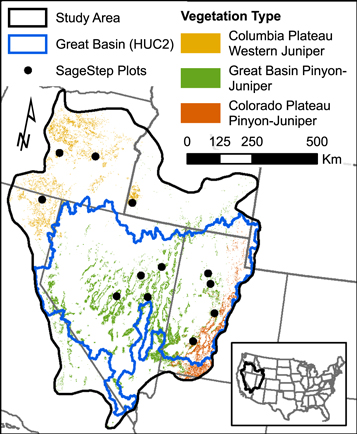
Figure 1. Study area (736 500 km2) and mask of woodlands used for cover and biomass mapping derived from Landfire Existing Vegetation Type (LF2.0.0), and clusters of SageSTEP plots used for validation of canopy cover estimates.
Download figure:
Standard image High-resolution imageWe limited our temporal extent to 2000–2016 to match the availability of consistently measured FIA data which we use as a basis of comparison. In 1999 FIA began transitioning from periodic independent collections in each state to collecting a portion of plots annually with a consistent sampling design.
2.2. Remotely sensed data
Falkowski et al (2017) produced a high-resolution map of canopy cover across the greater sage-grouse range by applying spatial wavelet analysis to National Agriculture Image Program (NAIP) imagery collected between 2011 and 2013. Spatial wavelet analysis, also known as Laplacian of Gaussian blob detection, identifies the location and size of bright circular objects against a dark background by convolving a single band image with a Mexican hat wavelet of several radii to produce a scale-space transform of the image which is searched for local maxima. Canopy cover, defined as the percent vertical projection of tree crown area (Jennings et al 1999), was calculated from tree crowns identified by this algorithm by gridding percent tree crown area at scale of 30 m. This canopy cover map overlaps most of our study area and served as a basis for model training and validation in our efforts to map PJ canopy cover from 2000 to 2016. Along with the Landsat imagery, topographic indices generated from the National Elevation Dataset (10 m) and variables derived from contemporary climate surfaces (Rehfeldt 2006) were incorporated into models of canopy cover.
2.3. Sampling
The canopy cover map produced by Falkowski et al (2017) was stratified into 5% cover intervals (0%, 1%–4%, 5%–9%, 10%–14%, etc) and randomly sampled in a GIS at a rate of 1 sample per 1000 km2 per class, which produced 5458 samples. This stratified random sample of cover enabled high cover values, which were rare on the landscape, to be represented in the model training data. The delineated tree crowns for each 30 m × 30 m sample of canopy cover were compared against the aerial imagery used to produce it, and only samples which appeared to accurately represent the canopy were retained for model training (n = 2535). This method is a rapid semi-automated approach which enables more samples to be gathered than could be obtained from using a dot-grid or field measurements but ensures cover estimates are more accurate for model training than if the automated tree extraction were fully relied upon. Training samples may have been biased towards tree configurations that were more easily captured by spatial wavelet analysis, but the accuracy of modeled canopy cover derived from this approach was evaluated with independent field data.
2.4. Image and topographic data preparation
Landsat Tier 1 Surface Reflectance imagery was cloud masked before producing temporal composites of spectral indices which were used as input for the LandTrendr Algorithm in Google Earth Engine (Kennedy et al 2018). Initial tests revealed a date range of 22 September–22 December best captured coniferous tree canopy cover while minimizing the influence of background vegetation which is predominantly senesced in autumn. Images in this date range were collected from 1998 to 2017 to provide a temporal buffer for LandTrendr segmentation, which can often fail to identify significant changes in the first or last year of a time series. The influence of clouds, cloud shadows, and snow was minimized by discarding images with greater than 50% cloud cover and masking the remaining occluded pixels with the included CFMask band (Foga et al 2017). Landsat-8 images were harmonized to Landsat-7 to improve continuity between the sensors (Roy et al 2016). The Normalized Difference Vegetation Index (NDVI; Rouse et al 1974), Normalized Burn Ratio (NBR; Key and Benson 2006), and Normalized Difference Moisture or Water Index (NDMI; Gao 1996), and Enhanced Vegetation Index (EVI; Liu and Huete 1995) were produced for each image (table S1, available online at stacks.iop.org/ERL/15/025004/mmedia). The annual median pixel value for each spectral index and band (table S1) was obtained to produce annual composites. These annual composites were temporally segmented with the LandTrendr algorithm (Kennedy et al 2010) using a maximum of 6 segments, a spike threshold of 0.9, a p-value threshold of 0.05, recovery threshold of 0.35, and a best model proportion value of 0.75. These parameters were selected from initial tests which involved visualizing the segmentation of pixel time series for areas with a variety of cover values and disturbance histories. The resulting fitted annual values of spectral indices and bands from the temporal segmentation, along with topographic and climate data, were used in modeling of canopy cover.
The topographic indices were produced from the National Elevation Dataset and included elevation, percent slope, the cosine and sine of aspect, the interaction of slope with the cosine and sine of aspect (Stage 1976), the solar-radiation aspect index (Roberts and Cooper 1989), the topographic position index calculated at scales of 90 and 990 m (Weiss 2001), the continuous heat-insolation load index (Theobald et al 2015), and the topographic diversity index (Theobald et al 2015). Biologically relevant climate variables as calculated by Rehfeldt (2006) were derived from 30-year climate normals (1981–2010) downscaled to 30 m. The initial climate surfaces were produced by fitting thin-plated spline models to weather station monthly averages of temperature and precipitation and interpolating these models to a 30 m grid with the shuttle radar topographic mission digital elevation model. Derived climate variables included 30-year normals of growing season precipitation, frost-free period in days (ffp), and others listed and described in table S1.
2.5. Canopy cover mapping
Canopy cover was mapped annually at a 30 m resolution for all PJ woodlands in the study area from 2000 to 2016. LandTrendr fitted bands, topographic indices, and climate variables served as predictors of the canopy cover samples derived from the Falkowski et al (2017) map in a Random Forest model (Breiman 2001). The model of 2535 samples used 250 decision trees, and the square root of the total number of variables (n = 40; table S1) was considered when splitting at each node. In addition to external validation with field data, we evaluated model fit from out-of-bag predictions which produce unbiased estimates of error (Breiman 2001). Cover maps were masked to the extent of PJ woodlands in the study area to prevent overestimation of PJ cover in other ecosystems. The extent of PJ woodlands was mapped by reclassifying the 2016 Landfire Existing Vegetation Type dataset (LANDFIRE 2016) with the following vegetation type classes included in the PJ mask (class codes in parentheses): Great Basin PJ Woodland (7019), Columbia Plateau Western Juniper Woodland and Savanna (7017), Colorado Plateau PJ Woodland (7016), Colorado Plateau PJ Shrubland (7102), Rocky Mountain Foothill Limber Pine-Juniper Woodland (7049), Inter-Mountain Basins Juniper Savanna (7115). The resulting aggregated class had a user's accuracy of 64% and producer's accuracy of 73% as determined from the contingency tables produced for the Southwest and Northwest regions (https://landfire.gov/remapevt_assessment.php, accessed 6 September, 2019). We also compared this mask to independent FIA plots measured in 2016 which had at least one condition labeled as a PJ forest type; this comparison yielded a user's accuracy of 71% and producer's accuracy of 62%. Since the PJ extent as determined by LANDFIRE is derived primarily from 2016 imagery, it may exclude PJ which existed within our timeframe of interest (2000–2016) but was completely removed by disturbance prior to 2016.
2.6. Biomass mapping
From the maps of canopy cover we produced annual maps of biomass for the same time period (2000–2016). Due to the short stature of PJ woodlands, biomass can be mapped directly from canopy cover without the saturation problems that occur in most forests at high levels of cover. We used tree crown-based allometrics (section S1) for Utah juniper, single-leaf pinyon, and western juniper (Sabin 2008, Tausch 2009, Campbell et al 2012) to obtain plot-level biomass in Underdown Canyon, Nevada (Rau et al 2012) and the Owyhee Plateau, Idaho (Strand et al 2008). Plot-level biomass was regressed against percent canopy cover (equation (1)) which shows aboveground biomass (AGB in Mg ha−1) has nearly a one-to-one relationship with percent canopy cover (c) for both western juniper and Great Basin PJ ecosystems (R2 = 0.98, RMSE = 3.68 Mg ha−1, n = 67).

Details of this allometric relationship and its comparison to FIA allometrics may be found in section S1. Applying this allometry to maps of cover rather than modeling field biomass directly introduces little error, enables mapping of both cover and biomass, and allows the remote sensing model to be constructed with a much larger representative sample (n = 67 versus n = 2535).
2.7. Field Validation
2.7.1. Sagebrush steppe treatment evaluation project data
We compared predictions of canopy cover to field measurements gathered as part of the Sagebrush Steppe Treatment Evaluation Project (SageSTEP; McIver et al 2014). SageSTEP conducted experiments on several sagebrush restoration treatment methods across the Great Basin in 2005–2010 centered within our study period and with 178 control plots (i.e. no treatment) clustered in 12 sites coinciding with our study area. Field data collected for each rectangular 30 m × 33 m plot in 2006 and 2007 included measures of crown diameter for each tree from which we calculated plot-level percent canopy cover.
2.7.2. Forest Inventory and analysis data
Predicted aboveground biomass was also compared to biomass estimates from the USFS Forest Inventory and Analysis program (FIA) at the plot and county levels. Plots overlapping the study area and timeframe which contained greater than 50% of their biomass in the following PJ species were included in the plot-level comparison: Utah juniper, western juniper, Rocky Mountain juniper (Juniperus scopulorum Sarg.), one-seed juniper (Juniperus monosperma (Engelm.) Sarg.), alligator juniper (Juniperus deppeana Steud.), California juniper (Juniperus californica Carr.), single-leaf pinyon, two-needle pinyon (Pinus edulis Engelm), Arizona pinyon (Pinus monophylla var. fallax Little). For plot-level comparisons, predictions were extracted from our annual maps of biomass in the year each plot was measured by FIA at the true plot coordinates. Annual correction factors (equation (2)) were calculated based on this plot-level comparison and applied to the biomass maps for all subsequent analyses (see section S2):

where c is the correction factor and y is year. For county-level comparisons, FIA estimates of total county biomass were calculated using the standard population-level estimation procedures provided through the EVALIDator tool for the most recent inventory in each state and using the FIA definition of PJ forest (USFS 2019). Since FIA does not measure all 'non-forest' plots (i.e. plots with less than 10% cover), we excluded pixels with less than 10% cover when making county-level comparisons to the maps. We maintain these definitions of 'forest' (i.e. ≥ 10% cover), 'non-forest' (i.e. < 10% cover), and the more general 'PJ woodlands' (>0% cover) in subsequent analyses.
2.8. Analysis of cover and carbon trends
Maps of canopy cover and biomass were used to analyze trends across the entire study area. We examined the change in total aboveground biomass and forest area over time. We also investigated how much of the change in biomass can be attributed to an increase in forest area (i.e. increase to ≥10% cover), infilling of existing PJ woodlands, and canopy cover loss. For losses, we tallied the change in biomass which could be attributed to wildfire as determined from the Monitoring Trends in Burn Severity dataset (USFS/USGS 2018). Since our mapping and analysis was limited to areas classified as PJ in the final year of our time series, many areas with prior disturbance and a change in land cover type were likely excluded. To examine the potential impact of these disturbances on our estimates of change in biomass, we totaled the area and biomass change over excluded PJ areas which experienced a disturbance between 2011–13 and 2015–17 as mapped by Reinhardt et al (in press).
3. Results
The canopy cover model had an out-of-bag R2 of 0.75 and RMSE of 8.77% cover and exhibited a mostly even distribution of residuals with some overestimation when observed cover was below 10% and underestimation when observed cover exceeded 50% (figure 2(a)). Plot-level validation of canopy cover against SageSTEP had a similar accuracy and distribution of errors to the out-of-bag comparison (figure 2(b), R2 = 0.67, RMSE = 10.17% cover). The short-wave infrared-based spectral indices (NBR and NDMI) were the top two important features in the random forest model of cover followed by spectral indices of vegetation greenness (NDVI and EVI) (figure S4). The Continuous Heat-Insolation Load Index (chili) and summer precipitation (smrp) were the top ranked topographic and climate variables, respectively, but still had lower importance than most Landsat-derived variables. Even though predicted biomass had an apparent strong linear relationship to FIA plot biomass (figure 3), FIA biomass was 4.93 Mg ha−1 lower on average, which led to low R2 and high RMSE values. This bias and apparent lack of fit can be largely attributed to differences in tree-level allometry between the crown-based approach used in this study and FIA's Component Ratio Method as discussed in section S1. County-level estimates of biomass closely matched those from FIA following correction for plot-level bias (R2 = 0.97, figure 4). Over the whole study area, PJ forest biomass totaled 171 Tg according to 2016 FIA inventories, which was 21% of the total forest biomass (USFS 2019). By comparison, our 2016 map of PJ biomass estimates 161.6 Tg on PJ forest land (i.e. ≥10% cover) and 163.0 Tg when including 'non-forest' biomass (i.e. <10% cover). This difference can mostly be attributed to the Landfire-based mask of PJ forest area comprising 89% of the area estimated by FIA in 2016, despite the forest areas closely matching on a county-level (R2 = 0.97; figure S5).

Figure 2. Comparison of out-of-bag predictions of canopy cover from the random forest model against spatial wavelet analysis estimates of canopy cover used for model training (a). Comparison of cover predictions with field estimates from SageSTEP (b). R2, RMSE, and bias are given with respect to the 1:1 line (dashed black).
Download figure:
Standard image High-resolution image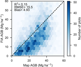
Figure 3. Hexbin (2D histogram) of predicted biomass compared to FIA plot biomass (n = 4241); R2, RMSE, and bias are given with respect to the 1:1 line (dashed black). Apparent bias and lack of fit is largely due to differences in tree-level allometrics between the crown-based approached used for mapping and FIA's component ratio method (section S1).
Download figure:
Standard image High-resolution image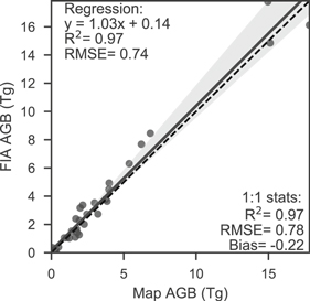
Figure 4. Comparison of map biomass to FIA county biomass for the most recent inventory of each state. Accuracy statistics are given with respect to the regression line (solid black) and 1:1 line (dashed black).
Download figure:
Standard image High-resolution imageFrom 2000 to 2016 PJ biomass increased by 9.86 Tg with a steady increase of 0.39% per year on average (figure 5). The changes in biomass varied spatially, with 5.1% and 1.2% of the study area increasing and decreasing, respectively, by more than 10 Mg ha−1 (figure 6). Woodlands dominated by western juniper in the Columbia Plateau had a higher average rate of biomass increase (0.98%) compared to PJ in the Great Basin (0.21%) or Colorado Plateau (0.48%). The overall increase in biomass was mostly attributed to infilling of existing 'forest' areas (≥10% cover) rather than expansion of PJ into sagebrush or grassland with <10% tree cover (figure 7), even though forest area increased by 4610 km2 at an overall rate of 0.46% per year (figure 8). Over the entire time span of this study, 33 603 km2 experienced infilling totaling 14.2 Tg in comparison to the 3.47 Tg that can be attributed to expansion (i.e. increase in cover to ≥10%). A total of 8 Tg of biomass was lost in other areas (28 736 km2) with wildfire responsible for approximately one-tenth of the decrease (0.81 Tg over 1278 km2) as determined from the change in biomass within wildfires captured by the Monitoring Trends in Burn Severity dataset. The remaining loss was likely due to management, development, or extreme drought. The PJ mask excluded 1753 km2 of areas classified as disturbed between 2011–13 and 2015–17 by Reinhardt et al (in press), which would have accounted for an additional loss of 1.42 Tg.
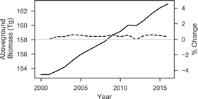
Figure 5. Total aboveground biomass over time (solid line, left axis) and the percent annual change (dashed line, right axis).
Download figure:
Standard image High-resolution image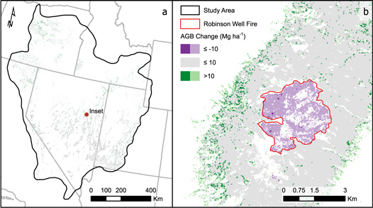
Figure 6. Map of change in biomass between 2000 and 2016 for the full study area (a) with close-up view of the 2001 Robinson Well fire (b). Significant increases in biomass (>10 Mg ha−1) generally occurred on the edges of current PJ while decreases occurred in areas of disturbance. Lighter shades, such as the majority of the burn area, indicate areas of change captured by the model but excluded by the Landfire-based PJ mask due to a change in land cover classification.
Download figure:
Standard image High-resolution image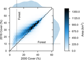
Figure 7. Hexbin (2D histogram) and marginal histograms of canopy cover in 2000 and 2016. Forest is defined as areas with at least 10% cover.
Download figure:
Standard image High-resolution image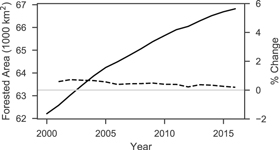
Figure 8. Forested area (i.e. ≥10% cover) over time (solid line, left axis) and the percent annual change (dashed black line, right axis).
Download figure:
Standard image High-resolution image
4. Discussion
Even after 150 years of prior encroachment, PJ is continuing to replace sagebrush and grasslands with 4600 km2 of new 'forest' (i.e. ≥10% tree cover) between 2000 and 2016 despite some loss of forest from management and various disturbances. Rates of encroachment have been reported to decrease in the latter half of the 20th century (Miller et al 2008) with landscape scale studies showing increases in cover of 0.4%–1.5% per year since the 1960s (Sankey and Germino 2008). These rates may have been expected to decline further as areas suitable for PJ establishment diminish, but we find encroachment into non-forest areas from 2000 to 2016 continuing at an overall rate of 0.46% per year (figure 8) and an average increase in percent canopy cover of 3.9%. Losses of biomass from management, wildfire, and other disturbances comprised extensive reductions (8 Tg) but were still not enough to offset increases in other areas (17.8 Tg). However, limiting the extent of our analysis based on 2016 land cover excluded at least 1.42 Tg of biomass loss that occurred between 2011–13 and 2015–17, and further losses in prior years were likely excluded as well. It is uncertain if the overall trend of increasing cover and biomass will continue, as areas suitable for establishment of PJ may in fact be diminishing. Some existing woodlands may also be reaching a carrying capacity which limits further infilling due to resource constraints. Projections also indicate increased future potential for wildfire and extreme drought (Breshears et al 2005, Buotte et al 2019), which may offset increases by encroachment and infilling. In addition to losses by natural causes, there has been increased investment in PJ removal in recent years for restoring greater sage-grouse habitat (Natural Resources Conservation Service 2015). Indeed, the National Environmental Policy Act (NEPA) exclusions for PJ removal in the 2018 Farm Bill will enable further PJ removal and sagebrush restoration in the near future (Conaway 2018). For example, the proposed Bruneau-Owyhee Sage-grouse Habitat Project would remove western juniper from 294 000 ha in southwestern Idaho (Bureau of Land Management 2018). The large investment in sagebrush restoration presents an opportunity to not only increase habitat for greater sage-grouse but to also manage PJ stands for increased resilience to the impacts of a changing climate such as extreme drought and large-scale wildfires.
The trend of increasing PJ biomass (figure 5) could make PJ woodlands an important component of national carbon accounting efforts and certainly has widespread implications for biodiversity and ecosystem services, even though PJ systems represent a modest fraction of forest biomass in the western USA according to FIA (e.g. 21% within our study area). PJ encroachment may also cause a small increase in belowground organic carbon (Rau et al 2011) which we did not account for in this study. Despite the potential significance of PJ systems for carbon accounting, much of the PJ biomass is excluded by FIA and thus also excluded from the EPA's Greenhouse Gas Inventory reporting, which does not currently estimate woody biomass on rangelands where there is low canopy cover (EPA 2019). In the Great Plains trees outside of forests account for nearly half of the treed area (Meneguzzo et al 2018), and such non-forest areas with trees may comprise a large portion of the Great Basin as well. Unfortunately, commonly used land cover maps and forest masks often exclude low cover areas. This may explain the decrease we observed in non-forest area (i.e. <10% cover) from 8.1% of the study area in 2000 to just 1.3% in 2016 (figure 7); as the 2016 land cover map may have failed to capture areas of recent PJ encroachment. Surveying and improvements in remote sensing of trees outside of forests could provide a more complete picture to carbon accounting efforts (Johnson et al 2015).
In addition to carbon accounting, tracking of PJ cover and biomass could enable landscape- to regional-scale monitoring of potential changes to biodiversity and ecosystem services which are known to accompany PJ cover dynamics. Indeed, the continued expansion (7% of study area) and infilling (50% of study area) of PJ forest over the region suggests that some of the known consequences of encroachment, such as decreased water availability (Roundy et al 2014, Kormos et al 2017) and herbaceous plant diversity (Miller et al 2000), are likely widespread. The high degree of infilling of existing PJ woodlands we observed (figure 7) also poses an increased risk of high severity fires (Miller et al 2008, Romme et al 2009), which may subsequently increase the risk of cheatgrass (Bromus tectorum L.) invasion in sites with a low resistance to invasion (Williams et al 2017, Davies et al 2019).
By applying the LandTrendr algorithm to Landsat imagery in Google Earth Engine, we were able to rapidly produce stable estimates of PJ biomass over a broad region for over a decade. However, by scaling estimates of cover from aerial imagery to Landsat we introduce additional error (out-of-bag RMSE = 8.77% cover) and lose the potential utility provided by individual tree measurements and high-resolution maps. Our approach is also based on the assumption that harmonizing sensors and using the LandTrendr segmentation algorithm enables a single model to be applied across the entire time series with consistent accuracy (Vogeler et al 2018). However, validating and quantifying uncertainty for annual maps would provide a check of this assumption and enable propagation of uncertainty to subsequent analyses. Future efforts could also implement annual mapping of woodland extent rather than using a single mask, which could better capture early stages of encroachment and avoid exclusion of previous woodlands which experienced a change in land cover. These improvements would create an approach that could potentially be applied in many other woodlands for robust MRV of woody carbon to meet the needs of national carbon accounting efforts and aid land management.
5. Conclusion
A system for regional scale monitoring of woody cover and biomass is needed for the world's dryland biomes due to their vast area, high degree of change, and the implications of that change for carbon storage, biodiversity, wildfire risk, and ecosystem services among other concerns. Here we demonstrated a carbon monitoring system for PJ woodlands in the western United States, which is scalable to large regions with annual frequency through the combination of sampling from VHR imagery, trend-fitting of Landsat time series to capture annual cover dynamics, and cover-based allometry to estimate biomass. Through this approach we found biomass continuing to increase at an average rate of 0.39% per year from 2000 to 2016, with 80% of the total increase attributable to infilling of existing woodland areas with ≥10% tree cover—the cover threshold used by FIA in defining forest. While in this paper we only investigate historical trends in cover and biomass, regional time series such as these may also be beneficial for projecting future changes in drylands such as susceptibility to woody encroachment or vulnerability to the effects of climate change. This prototype carbon monitoring system could easily be extended to similar woodlands around the world to improve monitoring of carbon storage, understand the impacts of historic changes in woody structure, and prepare for future change.
Acknowledgments
This work was funded by NASA Carbon Monitoring System Award #NNH15AZ06I awarded to Principal Investigator Andrew Hudak and through a Joint Venture Agreement from the USFS Rocky Mountain Research Station to Colorado State University (16-JV-11221633-061). We would like to thank Bethany Bradley for connecting us with the Sagebrush Steppe Treatment Evaluation Project which contributed essential field data (Contribution Number 133). Thanks also to Robert Kennedy, Warren Cohen, and Sean Healey for providing early access to the Google Earth Engine implementation of LandTrendr.
Data availability statement
The data that support the findings of this study are openly available through the Oak Ridge National Laboratory Distributed Active Archive Center at DOI:10.3334/ORNLDAAC/1755.