

Abstract
Social, technological and climatic changes will transform the way energy is consumed over the 21st century, with important implications for energy networks and greenhouse gas emissions. Here, we develop a method to efficiently explore climate-energy interactions under various scenarios of climate, urban infrastructure and technological change. We couple the Urban Climate and Energy Model with the Conformal Cubic Atmospheric Model as a full-height single column driven with a series of global climate model simulations in an ensemble approach. The framework is evaluated against observations, then a series of century-scale simulations are undertaken to examine projected climate change impacts on electricity and gas demand in the temperate/ oceanic climate of Melbourne, Australia. With air-conditioning ownership remaining at early 21st century levels, and in the absence of other changes, climate change under radiative forcing RCP 8.5 increases peak electricity demand by 10%, and decreases peak gas demand by 22% between 2000 and 2100. However, if projected increases in air-conditioning ownership are considered, peak electricity demand increases by 84%, surpassing peak gas demand in the second half of the century. These findings highlight the complex nature of changes facing energy networks. Changes will be location and scenario dependent.
Export citation and abstract BibTeX RIS

Original content from this work may be used under the terms of the Creative Commons Attribution 3.0 licence. Any further distribution of this work must maintain attribution to the author(s) and the title of the work, journal citation and DOI.
1. Introduction
In 2018 the International Energy Agency (IEA) declared the rapid growth of electricity demand from air conditioners (ACs) as 'one of the most critical yet often overlooked energy issues of our time' (IEA 2018). The demand for cooling has recently grown to now consume about 10% of electricity globally, and the IEA predict a further tripling of cooling demand between 2016 and 2050 without additional policy intervention beyond the 2015 United Nations Paris Agreement.
Increased energy consumption drives up greenhouse gas emissions, impacting global climate. Extreme weather and associated energy demand peaks challenge the reliability of energy networks, raising costs and risks for society (Zamuda et al 2013, Bartos et al 2016). In hot weather, more ACs are used and they become less efficient (Motta and Domanski 2000). The waste heat from their energy consumption is emitted into the atmosphere, further raising local air temperatures (Salamanca et al 2013, 2014). Studies across a range of world cities report peak electricity load increases between 0.45% and 4.6% per degree of ambient temperature increase, with an average increase of 2.65% (Santamouris et al 2015). In contrast, global warming will reduce building heating demands, although changes will be regionally and locally dependent (Santamouris 2014).
In many cities, energy demand for space heating is currently greater than the demand for cooling. This is the case for Melbourne, in the state of Victoria, Australia, located in a temperate/ oceanic climate under the Köppen–Geiger system (Beck et al 2018). For the period 2000–2009 the peak demand for gas in winter months was approximately double the peak demand for electricity in summer months when ACs were in use (figure 1). This relationship will change in the future as global warming leads to higher air temperatures and the number of households with air conditioning increases, significantly impacting energy supply network costs and greenhouse gas emissions (IEA 2018).

Figure 1. Electricity and gas demand (2000–2009) from state-level observations, scaled by population to energy use intensity in suburban Melbourne, Australia. See Lipson et al (2018).
Download figure:
Standard image High-resolution imageTo examine this climate-energy relation in Melbourne, we undertake a series of century-scale coupled building-urban-atmosphere simulations driven by global climate model (GCM) outputs under the high baseline Representative Concentration Pathway (RCP) 8.5 (Vuuren et al 2011).
1.1. A new modelling framework
Modelling climate-energy feedbacks is challenging because of the wide range of scales over which important processes interact. Meteorological conditions within cities are primarily affected by global and regional climate, however urbanisation also changes local conditions (McCarthy et al 2010). The radiative, thermal and mechanical properties of urban land surfaces, as well as the emission of anthropogenic heat as a by-product of energy consumption, results in local phenomena such as urban heat island, and micro-climate differences between streets and neighbourhoods (Hart and Sailor 2009, Theeuwes et al 2017). Energy consumption itself is affected by those local meteorological conditions, as a considerable proportion of energy is used for heating and cooling buildings (Pérez-Lombard et al 2008). This interrelation forms positive and negative feedbacks between local temperature and energy demand (Takane et al 2017, 2019).
Statistically-based studies, or those that use uncoupled warming projections to drive building energy models (BEMs), do not capture interrelated climate-energy feedbacks across all relevant scales. In order to capture these feedbacks, previous studies have integrated BEMs within urban canopy models (UCMs) to simulate urban-atmosphere energy and momentum flux exchange in numerical weather simulations (Kikegawa et al 2003, Salamanca et al 2009, Bueno et al 2012, Mauree et al 2017, Lipson et al 2018). Dynamically downscaling GCMs to regional and local scales and then coupling with an integrated BEM and urban canopy model in three-dimensional (3D) simulations will capture these feedbacks, but the approach is computationally expensive, limiting the range of climate variability and the variety of scenarios that can be sampled (Ortiz et al 2018). It is therefore beneficial to explore approaches which include interactions between global and regional climate, urban land use modification, waste heat emissions and energy demand, but reduce barriers of computational cost.
In order to more easily assess climate variability and urban development scenarios, this study explores climate-energy demand interactions using a single column model (SCM) in which land surface characteristics are altered between experiments. To achieve this, we couple an integrated building energy demand and urban land surface model (section 2.1) with a full-height atmospheric model (section 2.2) and nudge the atmospheric column with output from a range of global climate simulations (section 2.3) using Newtonian relaxation (section 2.4). The framework is evaluated against local flux tower observations (section 3) and then used in a series of century-long coupled building-urban-atmosphere simulations to study the effects of projected climate change on building energy demand in Melbourne, Australia.
2. Methods
2.1. The building energy-urban canopy model
The near-surface environment is simulated by the Urban Climate and Energy Model (UCLEM) (Lipson et al 2018), an extension of the Australian Town Energy Budget (ATEB) urban canopy model (Thatcher and Hurley 2012). ATEB and UCLEM were developed to represent Australian cities in regional weather and climate simulations. Together they are capable of predicting realistic air temperatures and winds (Thatcher and Hurley 2012), radiant and turbulent fluxes (Lipson et al 2017), and building energy demand variability (Lipson et al 2018). Since Lipson et al (2018), a number of model developments have further improved energy demand predictions when driven by local meteorology, and allowed the partitioning of electricity and gas demand separately (described in supplementary material is available online at stacks.iop.org/ERL/14/125014/mmedia).
2.2. The atmospheric model
Atmospheric fields are simulated by the Conformal Cubic Atmospheric Model (CCAM), a variable-stretched grid atmospheric GCM (AGCM) with a comprehensive set of scale-dependent parameterisations (McGregor 1996, McGregor and Dix 2001, 2008). CCAM is the primary tool used for dynamical downscaling and regional climate simulations by the Commonwealth Scientific and Industrial Research Organisation (CSIRO) in Australia.
CCAM uses the GFDL radiation scheme (Freidenreich and Ramaswamy 1999, Schwarzkopf and Ramaswamy 1999), with a prognostic cloud condensate scheme (Rotstayn 1997), a cumulus convection scheme (McGregor 2003), an eddy-diffusivity/mass-flux boundary layer scheme with k-epsilon closure (based on Hurley 2007), and land surface processes represented by the CABLE biosphere-atmosphere exchange model (Kowalczyk et al 2013). CCAM has been evaluated for near-surface air temperature and precipitation in the Australian region over 30 year periods (Thatcher and McGregor 2010, Di Virgilio et al 2019), and has been used in 21st century climate projections (Nguyen and McGregor 2012, Grose et al 2013, McGregor et al 2016). Original global simulations use CCAM version 1209, while later SCM simulations use CCAM version r4368.
2.3. GCM driving data
A series of global atmospheric simulations were run previously between 1961 and 2100 at approximately 50 km resolution by the CSIRO. Global simulations use CCAM with bias- and variance-corrected sea surface temperature (SST) fields (Hoffmann et al 2016) of six GCMs from the Coupled Model Intercomparison Project Phase 5 (CMIP5) (Taylor et al 2012) per the description in Katzfey et al (2016). The set of CMIP5 models (table 1) were chosen based on their ability to realistically capture observed rainfall, temperature, surface pressure and SSTs, along with cyclic oceanic features of the El Niño Southern Oscillation, important for Australian climate variability. Additionally, CMIP5 models that ranked highly but had similar SST warming patterns were excluded in order to better span uncertainty in future climate change projections.
Table 1. The six CMIP5 models chosen to represent future climate under RCP8.5. See Katzfey et al (2016) for details.
| CMIP5 model | References |
|---|---|
| CCSM4 | Gent et al (2011) |
| CNRM-CM5 | Voldoire et al (2013) |
| NorESM1-M | Bentsen et al (2013) |
| ACCESS1.0 | Bi et al (2013) |
| MPI-ESM-LR | Giorgetta et al (2013) |
| GFDL-CM3 | Griffies et al (2011) |
Previously run global outputs were available at 6 hourly intervals. Potential temperature, surface pressure, water vapour mixing ratio and wind vectors were linearly interpolated and used to nudge the SCM toward AGCM states.
2.4. Nudging in the single column framework
Nudging is often used in atmospheric simulations to better align model states with observations or larger domain host models. In 3D configurations, CCAM uses spectral nudging, which is scale-selective and can avoid spurious effects at regional boundary edges (Thatcher and McGregor 2009). However, spectral nudging is not appropriate in the current context as it depends on horizontal length scales not present in an SCM. Here we use another common method—Newtonian relaxation. Newtonian relaxation has been used extensively elsewhere, for example, to improve numerical weather prediction (Stauffer and Seaman 1990), to align regional downscaled simulations with a host model's dynamics (Uhe and Thatcher 2015), and to help evaluate parameterisations within SCM models (Lohmann et al 1999). We use it here to blend the emergent dynamics of a variable  within the SCM with the host model driving data:

where  is the timestep and
  is the relaxation time which controls the strength of the nudging towards the driving data. A relaxation time equal to the timestep means SCM state variables match exactly with GCM driving data. As the relaxation time increases, the land-atmosphere dynamics within the SCM more freely evolve, and consequently atmospheric states diverge from GCM simulations, and may become unrealistic. This trade-off between capturing land-atmosphere feedbacks and appropriate driving data is a drawback of using the less computationally expensive SCM framework. To evaluate errors of the SCM, we compare output with urban flux tower and energy demand observations for a one-year period (section 3).
Sensitivity analyses found the SCM performed reasonably well with 58 atmospheric levels and 10 min timesteps. For relaxation times above 1 h, near surface simulated and observed fluxes began to diverge, therefore relaxation time was limited to 1 h for all simulations (see supplementary material). Additionally, we found rainfall calculated by nudging the SCM was not consistent with current climatology, so in these simulations rainfall and cloud condensate are replaced by host GCM values without nudging. Other atmospheric prognostic variables were allowed to evolve according to equation (1).
3. Evaluation
3.1. Evaluation data
Evaluation is undertaken using flux tower observations over the low to medium density residential suburb of Preston, in Melbourne, Australia. Preston is a mid-ring suburb characterised by detached one-to-two story residential buildings and a mix of grass, shrubs and trees. Site location and morphology parameters used in all simulations are listed in table 2, with site characteristics further detailed in Coutts et al (2007a, 2007b) and Grimmond et al (2011). The land uses surrounding the flux tower are generally homogeneous, so simulations use a single urban morphology class description. A tiling approach is used to represent the different states of buildings with or without heating and cooling equipment within the same grid point. State variables for each tile evolve independently, with tile fluxes blended at the first atmospheric level at each timestep (refer to the supplementary material for further details).
Table 2. Single column model parameters. Urban morphology parameters are based on Grimmond et al (2011), building energy model parameters are based on Lipson et al (2018). Supplementary material contains details on AC efficiency/ coefficient of performance (COP) calculations.
| Simulation parameters | |
|---|---|
| Location | 145.014 E 37.731 S |
| Single column atmospheric levels | 58 |
| Driving data relaxation time | 1 h |
| Mean building height | 6.4 m |
| Street canyon height/width ratio | 0.42 |
| Vegetation footprint fraction | 0.38 |
| Building footprint fraction | 0.45 |
| Air change rate (infiltration) | 1.0 h−1 |
| Internal heat gain | 4.5 Wm−2 floor−1 |
| Internal comfort temperature | 22 °C ± 0 °C |
| Fraction of internal space with heating | 0.67 |
| Fraction of internal space with cooling | 0.25–0.67 |
| AC efficiency factor | 2 (COP ~3.6) |
Flux tower measurements were taken at 40 m, at a height considered representative of the neighbourhood rather than microclimate conditions closer to the ground (Coutts et al 2007b). Sampling rates were between 1 and 10 Hz, block averaged to 30 min intervals. Here, we isolate a one-year period from 28 November 2003 to 27 November 2004 (366 d) and compare with SCM data over the same period. Periods with missing observed data are not used in model analysis, with remaining sample numbers noted in corresponding figures.
To compare with 40 m observations, simulated 40 m values are diagnosed by linearly interpolated prognostic values from the nearest two atmospheric layers at each timestep. This is necessary as the atmospheric model uses a pressure-based vertical coordinate system where atmospheric level heights shift between timesteps.
Energy demand data are from state-level electricity and gas observations for Victoria, Australia, scaled by population density to energy use intensity in the Melbourne suburb of Preston (see Lipson et al 2018 for details). Electricity data were available at half-hour intervals, and gas data hourly (linearly resampled to half-hourly for analysis). Site morphology and internal building equipment parameters are shown in table 2. Urban material parameters are UCLEM defaults (see table S3 in supplementary material).
3.2. Evaluation results
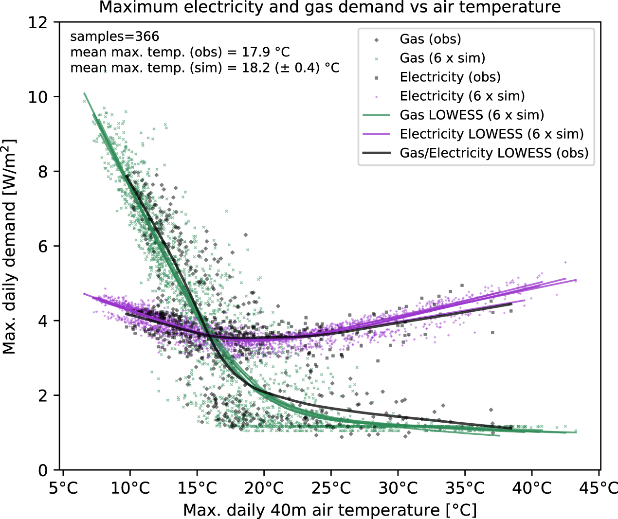
Figure 2 compares observed and modelled daily maximum 40 m air temperature with maximum gas and electricity demand for any time interval on that day. This gives a characteristic 'U' shaped electricity/temperature demand profile, where in cold weather more electricity is used for heating, and for cooling in hot weather. Gas is not used for cooling in hot weather, so is characterised by a more open 'L' shape. Locally weighted linear regressions (LOWESS) using 50% of closest data points are also shown. The modelled 40 m air temperatures are taken from the six CMIP5 driven SCM simulations and plotted with corresponding energy demand intensity for each GCM (resulting in six LOWESS lines). Individual weather events in simulated and observed systems will not match in time because simulations are driven by GCM projections, although the SCM should be expected to simulate the local climatology over longer periods. The observed maximum daily air temperature mean of 17.9 °C compares with an ensemble mean of 18.2 (standard deviation ± 0.4) °C.

Figure 2. Observed (obs) and simulated (sim) dependence of daily maximum electricity and gas demand on daily maximum 40 m air temperature in the one-year evaluation period. LOWESS lines indicate locally weighted average values. Text indicates the mean of observed daily maximum, and simulated ensemble mean and standard deviation over the year.
Download figure:
Standard image High-resolution imageFigure 2 shows that the SCM framework simulates a wider distribution of maximum daily air temperatures (both cooler and warmer) than observed over a 12 month period. This means that the SCM predicts larger hot and cold driven energy demand peaks for the 2003–2004 climate. The broader distribution is also likely because the six SCM simulations sample a more representative climatology than the 12 month observation period in which flux tower data is available. Notwithstanding these differences, average temperature and the LOWESS of observed and simulated data match well, therefore a shift in the distribution of temperatures should result in a reasonable shift in gas and electricity demand.
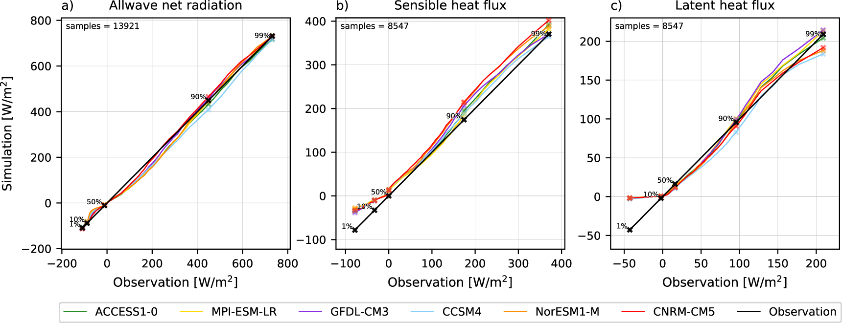
Figure 3 compares the observed and simulated distributions of radiative and turbulent heat fluxes at half-hour intervals using a quantile-quantile plot, with key percentiles highlighted with a cross in each distribution. All-wave net radiation is well simulated across the distribution, with the 1st, 10th, 50th, 90th and 99th percentiles closely matching observed values. Sensible heat flux is overestimated across the distribution for most simulations, particularly for negative observed values. Latent heat flux has a similar profile and is not able to capture observed negative values, however the 10th, 50th, 90th and 99th percentiles are reasonably captured. Overall, the evaluation indicates the framework can reasonably predict local climate and the variability in electricity and gas demand. This setup is next used in the 21st century control simulations presented below.
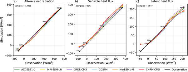
Figure 3. The distribution of simulated versus observed energy fluxes using a quantile-quantile plot over a one-year period for (a) all-wave net radiation, (b) sensible heat flux, (c) latent heat flux. Key percentiles are highlighted with a cross in each distribution and noted in text on the observed 1:1 line. The number of data points in each distribution is indicated in the top left-hand of each panel.
Download figure:
Standard image High-resolution image4. Results
Two experiments are presented, both consisting of six simulations of the CCAM+UCLEM SCM nudged by AGCM column output from global simulations, in turn driven by SSTs from six CMIP5 GCMs. The first experiment is a control, in which the RCP8.5 climate impact on energy demand is assessed by maintaining all land surface parameters at values used in the 2003–2004 evaluation, throughout the 21st century. A second experiment with rising AC accounts for a projected increase in ACs ownership.
4.1. Control experiment results
Figure 4(a) shows the climate impact on peak electricity and gas demand when the fraction of spaces with air conditioning is held at 0.25. The ensemble mean of yearly peak gas demand in the last decade of the 21st century is 21.8% lower (standard deviation ± 3.7%) than in the first decade, while yearly peak electricity demand increases by 10.3% (±2.9%). The total combined electricity and gas yearly mean demand decreases by 13.5% (±0.9%). Variability between ensemble projections are larger in peak demand projections compared with mean projections because the peaks are affected by the tails of temperature distributions, which are more variable.

Figure 4. Ensemble projections for yearly peak gas and electricity demand under RCP8.5 for (a) the control experiment and (b) the rising AC experiment, with mean combined (electricity + gas) energy demand also shown. The right axis shows both the percentage change in demand between the first and last decade for peak gas (green), peak electricity (purple) and mean energy (blue), along with the fraction of internal spaces with access to air conditioning in a given year (red). The first decade mean is based on control in both experiments.
Download figure:
Standard image High-resolution image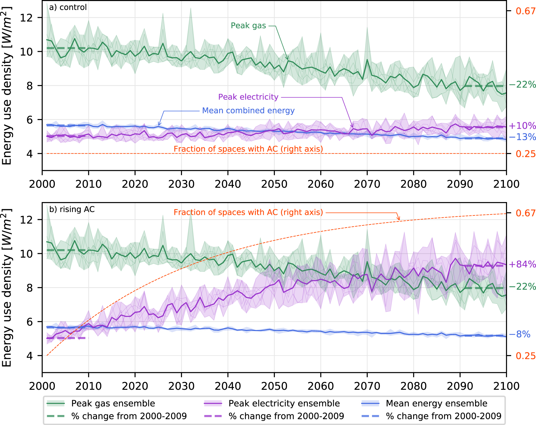
The simulated maximum daily 40 m air temperature in the first and last decade of the 21st century increased from 18.0 °C (±0.2 °C) to 22.0 °C (±0.7 °C). Gas and electricity energy demand is affected by changes in air temperatures, as indicated in figure 2. As the distribution of temperatures warm, less electricity is used for heating, and more is used for cooling. However, in the control experiment, the sign of the change in mean electricity demand differs from peak electricity demand. A summary of key rates of change in temperature and energy demand for the control experiment are presented in table 3.
Table 3. Ensemble mean and standard deviation (std) for key statistics in temperature and energy demand in the control experiment.
| Control experiment | Ensemble mean ± std |
|---|---|
| 2 m air temperature 2000–2009: | 15.2 °C ± 0.1 °C |
| 2 m air temperature 2090–2099: | 18.9 °C ± 0.4 °C |
| Local warming rate in RCP8.5: | +4.1 ± 0.4 °C/century |
| Electricity peak demand change: | +2.8 ± 0.7% per °C |
| Electricity mean demand change: | –0.4 ± 0.1% per °C |
| Gas peak demand change: | –5.9 ± 0.9% per °C |
| Gas mean demand change: | –8.0 ± 0.4% per °C |
| Combined mean demand change: | –3.7 ± 0.3% per °C |
4.2. Rising AC experiment results
A second experiment increases the fraction of internal spaces with air conditioning installed, from 0.25 to 0.67, which is equal to the proportion of spaces with access to heating (refer to supplementary material for information on increasing AC ownership and internal zoning assumptions). Figure 4(b) plots the resulting change in energy demand under RCP8.5.
In the rising AC experiment, the ensemble mean of yearly peak gas demand decreases again by 21.8% (±3.7%), however yearly peak electricity demand increases by 84.5% (±7.1%), while combined electricity and gas yearly mean demand decreases by 8.5% (±1.0%) overall. Variability between ensemble projections for peak electricity have a greater spread compared with the control experiment, increasing throughout the simulation period.
5. Discussion
This study highlights some of the complexities faced by energy networks under climate, technological and social change. Under RCP8.5, and in the absence of other changes, we found peak electricity demand in Melbourne increases by 10% over the 21st century, but if projected increases in air conditioning ownership are accounted for, peak demand increases by 84%. Peak electricity demand is important because it adds considerably to overall electricity network costs, and is critical for energy systems planning (Dirks et al 2015, Santamouris et al 2015). Our results suggest peak electricity demand is more sensitive to air conditioning installed capacity than to climate change itself. However, these drivers are interrelated. In cities of the United States, there is a strong correlation between warmer average temperatures and the number of installed ACs (Sailor and Pavlova 2003). Therefore, global warming is likely to drive an increase in air conditioning ownership, leading to an increase in electricity consumption, and in turn to increased greenhouse gas emissions.
The IEA predict a near quadrupling of air conditioning installed capacity between 2016 and 2050, primarily driven by economic, population and climate factors. This predicted increase accounts for already announced government policy aimed at curbing growth in energy use, including pledges made under the 2015 Paris Agreement. To mitigate this 'cold crunch', they suggest additional policy action is required, such as strong minimum energy performance standards in air conditioning and building construction, along with encouraging the use of photovoltaics and demand-side management (IEA 2018).
It is also important to highlight that increasing temperatures reduce heating demand, lowering energy costs and associated greenhouse gas emissions. Accounting for climate changes only, we found overall gas demand would decrease by –8.0% (±0.4%) per °C of warming, and electricity demand decrease by –0.4% (±0.1%) per °C. These results are based on suburban Melbourne, located in a temperate/ oceanic climatic region (Beck et al 2018) in which more energy is currently used to heat buildings rather than cool them. Large areas of Western Europe are also classed as temperate/ oceanic zones, and other regions of the world are cooler, but care must be taken in generalising results. Bartos et al (2016) examined projected climate change impacts on peak electricity load in the United States and found increases varied widely across the country, even within similar climatic regions. Peak load increases were not strongly correlated with the degree of regional temperature rise, but with the degree of urbanisation, AC ownership and usage patterns. The magnitude and even the sign of changes to overall or peak demand in electricity will be city-dependent. But overall, those cities with average temperatures to the right of the inflection point in their U-shaped electricity relation (figure 2) are likely to see significant increases in overall and peak electricity demand, while those to the left may benefit from some warming in terms of reduced mean electricity and other consumption.
A key finding in this study was that electricity peak demand in Melbourne will increase by +2.8% (± 0.7%) per 1 °C average temperature increase. This aligns with observational studies in a range of world cities which found on average an increase in peak electricity demand of 2.65% per 1 °C of ambient temperature increase (Santamouris et al 2015). In contrast, using a statistical regression demand model driven by GCM meteorological outputs, Thatcher (2007) found the peak regional demand in the state of Victoria (in which Melbourne is located) under a 1 °C increase would be –0.1% (±0.7%). A possible reason for the difference is the current study relies on an ensemble of climate projections. When analysed individually, the peak electricity demand of one of the six control simulations does decrease initially for 1 °C mean warming (at around 2030), then increases up to 2100. Peak demand is sensitive to the higher variability at the extremes of the temperature distribution, highlighting the advantage of the climate ensemble approach taken here.
Clearly, there are many factors in all urban environments that will change over a century, including population, building construction and urban form, air conditioning efficiency, network energy mix and partitioning into end uses, as well as human behaviours relating to energy use. This study is not intended to account for all possible changes, but to present a framework in which the impacts of these changes are able to be explored jointly with the impacts of a changing climate. The framework can be adapted for alternative scenarios, or to other regions, by taking the relevant atmospheric column and updating the UCLEM land surface parameters to account for local characteristics over time. The approach leverages previously run global climate simulations by reusing their output in a way that allows local dynamic interaction between the surface and the atmosphere.
Ensemble urban land-atmosphere studies at climate timescales are still rare in the literature, with some notable exceptions (e.g. Oleson et al 2018). Taking an ensemble approach allows quantification of the variability in climate projections. Multiple scenario modelling is also attractive in the urban context because potential paths of urban development are so diverse. The low computational overhead of an SCM provides value by allowing multiple scenarios to be easily modelled for a single land grid point.
Low computational overheads makes the SCM framework attractive, however the approach has drawbacks. The nudging method described in section 2.4 blends the dynamics from the GCM with those developing in the SCM, muting land-atmosphere feedbacks. We have assessed that a one-hour relaxation time provides an appropriate balance between land-atmosphere dynamics and GCM driving data, although the trade-off is subjective. Additionally, by its nature, an SCM cannot represent local 3D effects such as urban-induced advection flows (Barlow 2014, Fan et al 2018). Continental-scale 3D modelling studies have shown urban land surfaces raise near-surface temperatures in regions well outside urban extents (Georgescu et al 2014). These advected flows are not represented in an SCM, and so related land-atmosphere responses are not captured. In addition, as the SCM currently relies on GCM fields for rainfall it does not capture local precipitation feedbacks. As such, SCM simulations are not a replacement for fully-coupled 3D simulations, which can capture a broader range of land-atmosphere feedbacks. This framework provides value as it is a highly efficient method which can indicate first-order climate-energy feedbacks, and can be more easily used in ensemble studies to assess climate variability.
6. Conclusion
In this study we developed a single column building-urban-atmosphere framework which can explore cross-scale climate-energy interactions under various scenarios of global climate, urban planning, technological or human behavioural change. By coupling a BEM, an urban canopy model and a full-depth atmospheric model, driven by an ensemble of global climate projections, we are able to simulate the urban climate and building energy use for suburban Melbourne, Australia, through the 21st century under RCP 8.5. We find the climate change impact between the first and last decade of the 21st century is a mean increase in peak electricity demand of 10%, a decrease in peak gas demand of 22%, and a decrease in overall energy demand of 13%, all else held equal.
3D regional simulations include dynamics omitted in an SCM. The advantage of an SCM is that it can capture important climate-energy and vertical surface-atmosphere feedbacks at a much lower computational cost. SCM simulations took approximately 1.5 h per decade on a single processor. This easily enables an ensemble or range of simulations to be undertaken to explore the sensitivity of various physical systems, whether they be altered climate states, air conditioning ownership or efficiency, building construction or morphology, urban density or vegetation fraction changes. CCAM and UCLEM are open source.
Acknowledgments
This study was supported by the Australian Research Council (ARC) Centre of Excellence for Climate System Science (grant number CE110001028). The Commonwealth Scientific and Industrial Research Organisation (CSIRO) provided the global climate model host model data, which in turn relied on CMIP5 model SST outputs. We thank all groups for making their output available. Thanks to Dr Paola Petrelli for assistance in publishing associated datasets with the support of the ARC Centre of Excellence for Climate Extremes (grant CE170100023) and National Computational Infrastructure Australia. Thanks to Professor Sue Grimmond for discussions, and the University of Reading for support, while undertaking part of this work. Thank you to Professor Yuguo Li and Dr Alberto Martilli for providing valuable feedback on the thesis from which this study is based. Finally, thank you to the two reviewers for their feedback which improved the study.
Data availability statement
The data that support the findings of this study are openly available at: http://doi.org/10.25914/5d3e4a8074a5f.
NetCDF output files record surface variables at half-hour timesteps for the 2 × 6 century-scale simulations. Variables include radiation and turbulent heat fluxes, net storage heat flux, anthropogenic heat fluxes (including heating and cooling fluxes seperately), internal air temperatures (conditioned and unconditioned spaces seperately), precipitation, near-surface temperature and pressure, boundary layer height, cloud cover, 40 m air temperature, humidity and wind velocity.
The latest open source code for CCAM and UCLEM are available at: https://bitbucket.csiro.au/projects/CCAM/repos/ccam.