

Abstract
Reliable estimates of externality costs—such as the costs arising from premature mortality due to exposure to fine particulate matter (PM2.5)—are critical for policy analysis. To facilitate broader analysis, several datasets of the social costs of air quality have been produced by a set of reduced-complexity models (RCMs). It is much easier to use the tabulated marginal costs derived from RCMs than it is to run 'state-of-the-science' chemical transport models (CTMs). However, the differences between these datasets have not been systematically examined, leaving analysts with no guidance on how and when these differences matter. Here, we compare per-tonne marginal costs from ground level and elevated emission sources for each county in the United States for sulfur dioxide (SO2), nitrogen oxides (NOx), ammonia (NH3) and inert primary PM2.5 from three RCMs: Air Pollution Emission Experiments and Policy (AP2), Estimating Air pollution Social Impacts Using Regression (EASIUR) and the Intervention Model for Air Pollution (InMAP). National emission-weighted average damages vary among models by approximately 21%, 31%, 28% and 12% for inert primary PM2.5, SO2, NOx and NH3 emissions, respectively, for ground-level sources. For elevated sources, emission-weighted damages vary by approximately 42%, 26%, 42% and 20% for inert primary PM2.5, SO2, NOx and NH3 emissions, respectively. Despite fundamental structural differences, the three models predict marginal costs that are within the same order of magnitude. That different and independent methods have converged on similar results bolsters confidence in the RCMs. Policy analyzes of national-level air quality policies that sum over pollutants and geographical locations are often robust to these differences, although the differences may matter for more source- or location-specific analyzes. Overall, the loss of fidelity caused by using RCMs and their social cost datasets in place of CTMs is modest.
Export citation and abstract BibTeX RIS
1. Introduction
When analyzing policies, products or processes, it is critical to account for costs that are observed in the market as well as non-market costs, known as externalities (Baumol and Oates 1988). For air pollution, adverse human health effects—especially premature mortality from exposure to ambient concentrations of fine particulate matter (PM2.5)—result in large costs to society (US EPA 2009). To estimate these costs, the United States Environmental Protection Agency (US EPA) has generally employed an impact pathway assessment. This multi-step approach is as follows: first, chemical transport models (CTMs) are used to estimate the impact of emissions on ambient concentrations; second, the health effects from exposure to these concentrations are quantified using concentration–response (C–R) functions; finally, the health impacts are monetized. For premature mortality, an estimate of the willingness to pay to avoid this impact, known as the value of a statistical life (VSL), is used to monetize these impacts. At present, the US EPA employs a central estimate of USD 7.4 million (2006 values) (US EPA 2010).
The first step, modeling the relationship between pollutant emission and ambient PM2.5 concentrations, is especially challenging. PM2.5 consists of a complex mixture of chemical species, both inorganic and organic, from diverse sources. Some PM2.5 is emitted directly into the atmosphere and is referred to as inert primary PM2.5. Inert primary PM2.5 is dominated by particulate elemental carbon (PEC) and organic carbon (POC) (Hand et al 2012). However, most PM2.5 is secondary, meaning that it originates from gaseous emissions that react in the atmosphere to form products that condense into the particle phase. PM2.5 is also separated into its inorganic and organic components. Inorganic PM2.5 mostly results from emissions of sulfur dioxide (SO2), nitrogen oxides (NOx) and ammonia (NH3). These gaseous precursors are converted into sulfate ( ), nitrate (
 ) and ammonium (
 ) and form particulate matter through relatively well-understood chemistry. This chemistry, however, is highly nonlinear. The marginal sensitivities in PM2.5 concentrations to the precursor emissions depend on the initial concentrations and will change as the relative amounts of emissions of all three precursors change (Ansari and Pandis 1998). For example, recent trends in emissions have decreased the marginal effect of NH3 emissions and increased that of NOx emissions (Pinder et al 2008, Holt et al 2015). Organic PM2.5 consists of primary and secondary organic aerosol (POA and SOA, respectively) depending on whether it is emitted already in the particulate phase or whether it forms from gases in the atmosphere. SOA is formed from the oxidation of volatile organic compounds (VOCs), but the yield of organic PM2.5 varies substantially among VOC precursors. By contrast to the inorganic components, the sources and behavior of both POA and SOA are less well understood (Robinson et al 2007). While scientific understanding of the formation of organic PM2.5 is advancing rapidly, this updated understanding is still being incorporated into the CTMs, and thus into the resulting social costs. The major mechanism for removing PM2.5 is via precipitation. Hence, PM2.5 can be transported for several days downwind, affecting populations up to approximately 1000 km away from the point of emission (e.g. Evans et al 2002). On the other hand, primary PM2.5 emitted in urban areas will have a large impact in the immediate vicinity. As a result, models of PM2.5 must reproduce the behavior of a complex physical and chemical system, and they require both sufficiently high resolution near sources and a long-range spatial extent to capture all the health impacts of a single source.
CTMs are the 'state-of-the-science' tool for predicting how much PM2.5 is formed from a given set of emissions, but the complexity of these models limits their applicability. To improve the availability and accessibility of air quality modeling and cost estimates, air quality researchers have produced a set of new models, known as reduced-complexity air quality models (RCMs) and associated sets of marginal social costs, i.e. monetized damages per pollutant (in USD per tonne of emission). In this letter, we compare three RCMs and their datasets that provide estimates of externality costs from air pollution: the Air Pollution Emission Experiments and Policy (APEEP) model (Muller and Mendelsohn 2007) updated to AP2 (Muller et al 2011), the Estimating Air pollution Social Impacts Using Regression (EASIUR) model (Heo et al 2016a, 2016b) and the Intervention Model for Air Pollution (InMAP) (Tessum et al 2017). We select these three RCMs as they provide comprehensive estimates covering the entire continental United States (US) at relatively high spatial resolution (county level or finer).
In this inter-comparison, we have three main aims:
- i.To provide guidance on how and when the differences matter between these three RCMs. While these RCMs are documented in the peer-reviewed literature, the differences in the social cost datasets have not been systematically examined.
- ii.To compare the results from the RCMs with the CTMs. Since the RCMs are, by definition, less physically detailed than the CTMs, there is also a potential loss of fidelity. This type of comparison can help justify their use for certain applications and allow users to judge the robustness of the results from the RCMs.
- iii.To evaluate the uncertainty in the air quality models. While it is recognized that evaluating the uncertainty in the analysis of the benefits of air quality is critical, as the effects of changing PM2.5 levels on mortality constitute a key component of the US EPA's approach for assessing potential health benefits for air quality regulations (National Research Council 2002), characterizing the full uncertainty in the air quality model is especially challenging (e.g. Fraas and Lutter 2013). As the three RCMs take fundamentally different approaches to air quality modeling, they may be understood to produce largely independent estimates. Hence, comparing and quantifying the differences between the independently derived estimates of social costs from the RCMs also provides an indication of the uncertainty of how emissions are transformed into ambient concentrations.
2. Review of CTMs and RCMs for assessing the social costs of air quality
Predicting the impacts of emissions on ambient concentrations is usually done using a comprehensive CTM. CTMs are three-dimensional mechanistic models that predict ambient concentrations of pollutants using mass balance principles and accounting for emissions, transport and dispersion by winds, chemical transformations and atmospheric removal processes. CTMs are the most scientifically detailed and rigorous tools available for linking emissions to ambient concentrations. Examples of CTMs include the Comprehensive Air Quality Model with extensions (CAMx; ENVIRON 2016), the Community Multi-scale Air Quality model (CMAQ; Appel et al 2017) and the Weather Research and Forecasting model coupled with Chemistry (WRF-Chem; Powers et al 2017). Running full CTMs is very intensive in terms of expertize, time and resources so their use is generally limited to air quality researchers and regulatory authorities, such as the US EPA's regulatory impact assessment for revisions to the National Ambient Air Quality Standards (NAAQS) and state agencies as part of the accompanying State Implementation Plans (SIPs). Even then, many states do not have in-house capabilities to run CTMs, relying instead on consultants or regional associations for their modeling needs. Despite the availability of RCMs, however, it is prudent to use a full CTM to assess the likely impact of major air quality policies before their implementation to ensure the best estimates of benefits for comparison with costs. Additionally, the comprehensive CTMs constitute the benchmark against which simpler models can be judged.
A number of RCMs have been developed to address the challenges with running CTMs. The magnitude of the social costs of air pollution suggests the usefulness of models such as RCMs that facilitate the quantification of the costs and their uncertainty as part of routine policy analysis. Further, the availability of simpler and more accessible models expands the community of people who could quantify the public health costs of air pollution, including city planners, affected industries and citizen groups. Those who run CTMs can find RCMs useful when they want to quickly explore a broad range of emissions scenarios. Next, we describe and compare results from three such models which are described in detail below: AP2, EASIUR and InMAP. We also briefly describe other RCM efforts.
APEEP and its updated version, AP2, employ a source–receptor (S–R) matrix framework to map emissions to ambient concentrations at the county level (Muller and Mendelson 2007, Muller et al 2011). The contribution of emissions in a source county (S) to the ambient concentration in a receptor county (R) is represented as the (S, R) element in a matrix. In the module for PM2.5 formation, the model contains S–R matrices that govern how PEC, SO2, NOx, NH3 and VOC map to PM2.5. Each of these matrices accepts annual (US short tons per year) emission vectors to produces predictions of annual means. For each of these matrices, the model distinguishes between emissions released at four different effective height categories: ground-level emissions, point sources under 250 m, point sources between 250 and 500 m and point sources over 500 m. AP2 employs the approach to estimating the 
 and
and  equilibrium embodied in the Climatological Regional Dispersion Model (CRDM), a national-scale Gaussian dispersion model (Latimer 1996). In the equilibrium computations, ambient
  reacts preferentially with
  Second, ammonium nitrate (NH4NO3) is only able to form if there is excess
  To translate VOC emissions into secondary organic particulates, AP2 employs the fractional aerosol yield coefficients estimated by Grosjean and Seinfeld (1989). While APEEP was evaluated against a 2002 annual average baseline run produced by CMAQ, AP2 predictions are tested against Air Quality System (AQS) monitoring data. Calibration coefficients are used to adjust AP2 predictions to jointly minimize mean fractional error and mean fractional bias. We use AP2 in the text to clarify that we are comparing the results from the updated version of the original APEEP.
The EASIUR model (Heo et al 2016a, 2016b) estimates marginal social costs for four species—inert primary PM2.5, SO2, NOx and NH3—in a 36 km × 36 km grid covering the continental US. The social costs are provided for four seasons and for three emissions elevations (ground level, 150 m and 300 m). The EASIUR model was derived by running regressions on a CTM data set consisting of small emissions perturbations occurring at 100 sample locations. CAMx was run to calculate social costs of the four species at the sample locations (randomly chosen based on population size) across the nation. Then, the resulting per-tonne social costs were regressed as a function of exposed population and atmospheric variables such as temperature and atmospheric pressure using half of the sample locations as training for the regression and half as out-of-sample evaluations. Finally, using the regression models, per-tonne social costs were estimated at all the cells in the 36 km × 36 km grid. In addition, an EASIUR-based S–R model was developed from the regression results (Heo et al 2017). The S–R version was used to estimate concentrations for comparisons made in this study.
InMAP (Tessum et al 2017) combines simplified representations of atmospheric chemistry and physics with output from WRF-Chem to calculate annual average marginal changes in concentrations of PM2.5 caused by marginal changes in emissions of SO2, NOx, NH3, VOCs and inert primary PM2.5 using a three-dimensional spatial grid with horizontal resolution ranging between 1 km × 1 km in highly populated areas and 48 km × 48 km in unpopulated areas and over the ocean. InMAP operates independently of the underlying CTM, and InMAP users only need to also use a CTM or access the raw CTM output data if they are interested in applying InMAP to a new spatial or temporal domain (e.g. outside the continental US). An InMAP-based S–R matrix (ISRM; Goodkind et al 2019) was developed to estimate the health impacts and social costs of emissions in every InMAP grid cell at three emission heights (ground level, low stack-height point sources and high stack-height point sources). In the comparisons presented here, the social cost of emissions from county centroids are used.
There are other RCMs that we review here but do not include in our inter-comparison. The Co-Benefits Risk Assessment (COBRA) screening model, developed by the US EPA, provides marginal social costs at county-level resolution (US EPA 2018). COBRA and AP2 share the core framework for modeling the air quality impacts of a unit of emission. Both models are built around the CRDM (Latimer 1996) and then calibrated to existing air quality modeling and measurements. There are minor differences in the treatment of the elevated sources, the approach to the simplified chemistry and the calibration approach. Because COBRA and AP2 are built on the same core air quality modeling, marginal social costs from COBRA are typically very similar to those from AP2.
The US EPA's Response Surface Model (RSM), with its 'benefit per ton' values, is another similar tool (Fann et al 2009, Fann et al 2012, US EPA 2015). Compared with the RCMs evaluated here, RSM has lower spatial resolution, only providing average impacts for nine urban areas plus the US overall average. An advantage of RSM, however, is that it can capture some of the nonlinear responses in PM2.5 chemistry that can occur with larger changes in inorganic PM2.5 levels (e.g. Holt et al 2015). We also do not review related tools such as Environmental Benefits Mapping and Analysis Program (BenMAP), which is focused on estimating health outcomes and does not include any air quality modeling. Rather, it requires ambient concentrations as inputs rather than emissions (US EPA 2017). The RCMs evaluated in this letter use a similar approach to quantify the health effects and economic valuation as employed in BenMAP. Other studies have also provided marginal social cost values but for limited regions of the US or limited emissions sectors, including the Direct Decoupled Method (DDM) of Bergin et al (2008), regression-based approaches developed by Buonocore et al (2014) and Levy et al (2009), and source-based estimates from the Goddard Earth Observing System with Chemistry model (GEOS-Chem; Caiazzo et al 2013).
3. Methods and models
Here, we evaluate the performance and the damage estimates from three RCMs. One of the first applications of the RCMs has been to develop marginal damage estimates, i.e. those that result from small perturbations of emissions. The results from the model, expressed in USD of damage per tonne of emissions, are specified at a minimum for a type of pollutant, a location, a population and, at least implicitly, for a given time period (e.g. a year). All results in this letter are expressed in 2010 USD.
First, we assess the RCMs in terms of their ability to predict observed PM2.5 concentrations and their composition. We compared concentration estimates against annual average concentrations provided by US EPA's air data (available at https://www.epa.gov/outdoor-air-quality-data). A caveat is that, given nonlinearities in PM2.5 formation discussed above, one does not necessarily expect that the marginal values from the RCMs will predict realistic PM2.5 concentrations. Using the 2005 National Emissions Inventory (NEI), AP2 estimated concentrations directly using its county-level S–R model. By contrast, EASIUR and InMAP combined the 2005 NEI with each RCM's marginal damage estimates in a spatially disaggregated way, i.e. the emissions of each species in each model source location make a linear contribution to all model locations. These contributions are then summed at each downwind 'receptor' location to represent the RCM's prediction of PM2.5. The latter approach assumes that the nonlinearities in the chemistry are not large. As a representative CTM, we also show the performance for WRF-Chem (Grell et al 2005, as configured in Tessum et al 2015). Information on the configuration of WRF-Chem can be found in table S1.
Second, we conduct an inter-comparison of the social costs from three models, focusing on four main categories of emissions that form ambient PM2.5: inert primary PM2.5, SO2, NOx and NH3. To isolate the effect of the air quality modeling on the damage estimates, we harmonized the main inputs: baseline emissions, population, C–R function and VSL. We select the baseline emission inventories and population for 2005. For the PM2.5 C–R function, we use the results from the American Cancer Society (ACS) epidemiological study for annual, all-cause mortality for adults (Krewski et al 2009); we do not quantify morbidity effects. We apply the US EPA's VSL of USD 7.4 million (2006 USD). We do not show results for VOCs because EASIUR does not predict impacts from VOCs, due in part to the uncertainties described in section 1. Additionally, because neither AP2 nor InMAP accounts for the variability in SOA yield among individual VOC species, we are less confident that the variability between the models is representative of overall uncertainty in the predictions of SOA impacts than we are for the inorganic species. We discuss the implications of the uncertainty in the damage estimates and make recommendations for how to approach these estimates in section 4.
4. Results and discussion: comparison of ambient concentrations and social costs
First, we compare the models with WRF-Chem and find that, in general, they have similar performance. These results show some important trends, with all models, including the CTM, performing worse for  and
and  predictions, illustrating that some PM2.5 species are more difficult to model; by extension, the damage estimates for their precursors will be more uncertain. At the same time, the relative success in reconstructing PM2.5 concentrations from marginal impact estimates suggests that differences between marginal and average changes are not too large or mostly cancel out among different pollutants and locations. On balance, these comparisons boost confidence in the use of RCMs and suggest that the necessary simplifications inherent in them do not substantially degrade their performance compared with CTMs. EASIUR does not estimate damages or SOA formation from VOC emissions; hence, an estimate of total PM2.5 is not possible from EASIUR at the present time. Additionally, we do not include a comparison of InMAP's predicted PEC concentrations against observations. In principle, InMAP can predict PEC; however, the NEI only reports total primary PM2.5. It is outside the scope of this work to conduct the additional processing to speciate these emission into InMAP format. We show the results of this evaluation in the supplemental information (figure S1). In addition to this comparison with WRF-Chem, each RCM has undergone substantial validation to both CTMs and, in the case of AP2, observed ambient concentrations. InMAP was compared against 14 separate runs from WRF-Chem to show that it could predict concentration changes (Tessum et al 2017). EASIUR was directly derived from the output of CAMx with out-of-sample evaluations for independent testing and is thus already indirectly validated against a CTM. Further, by comparing AP2 and InMAP with EASIUR, they are also indirectly compared with CAMx.
Turning to social costs, figure 1 shows the summary results for ground and elevated sources in the US. For ground-level sources, emission-weighted damages for the US varied by approximately 21%, 31%, 28% and 12% for inert primary PM2.5, SO2, NOx and NH3 emissions, respectively, with a range of 70 000–120 000 USD per tonne of PM2.5, 21 000–45 000 USD per tonne of SO2, 6400–13 000 USD per tonne of NOx and 38 000–49 000 USD per tonne of NH3. For elevated sources, emission-weighted damages for the US varied by approximately 42%, 26%, 42% and 20% for inert primary PM2.5, SO2, NOx and NH3 emissions, respectively with a range of 36 000–110 000 USD per tonne of PM2.5, 20 000–35 000 USD per tonne of SO2, 6300–11 000 USD per tonne of NOx, and 32 000–51 000 USD per tonne of NH3. Table S2 in the supplemental information tabulates values and calculations of variance. We report emissions-weighted averages, because aggregate health damages from a set of emissions are the sum of the emissions rate and marginal social cost which is then summed across all source locations. Therefore, aggregate damages are proportional to the emissions-weighted mean. Put another way, if two models differ by 10% in their emissions-weighted mean, their assessment of aggregate damages across the country for that species would also differ by 10%. Therefore, this metric is a good indicator of how much two models would differ for a policy where emissions changes are distributed similarly to current emissions. We also compare our national results with those produced by Fann et al (2009). We find that our values are within the same range, with the exception of primary PM2.5 where Fann et al (2009) have much higher values than the three RCMs. We show the tabulated comparison in table S3.
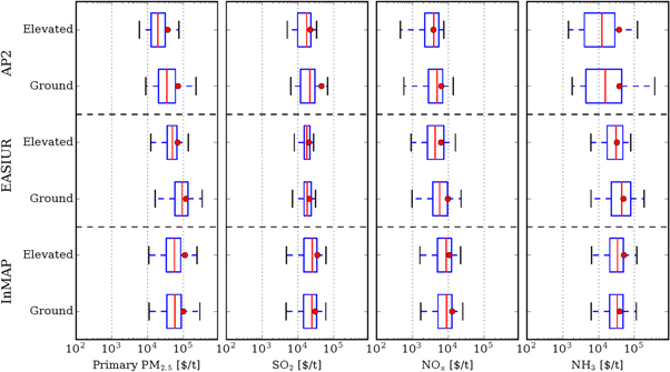
Figure 1. Box plot of the marginal social costs (in USD per tonne) for ground and elevated source emissions across all US counties by pollutant and by air quality model. Red dots and lines indicate emission-weighted mean and median, respectively. The left and right boxes are the 25th and 75th percentiles and the whiskers are the 2.5th and 97.5th percentiles. See table S1 for tabulated values.
Download figure:
Standard image High-resolution imageOverall, these three sets of marginal costs show similar trends. First, as shown in figure 1, for any given emitted species by model, the marginal social cost varies by at least one order of magnitude depending on the location of emissions for both ground and elevated sources. Additionally, we conclude that the elevated and ground-level sources generally behave the same, with most point sources having a similar or lower social cost than the ground-level sources. While the elevation allows the plume to span a greater area, the point sources are generally in rural areas. There are isolated cases where the reverse is true. These exceptions occur where the point sources, which are primarily in rural areas, have plumes that overlap with highly populated urban centers. Furthermore, the difference between elevated and ground is largest for primary PM2.5, as expected. For secondary PM2.5, where chemical and physical transformation needs to take place, the social costs are similar. By the time the PM2.5 is formed by chemical reactions, there has been enough vertical mixing that the original release height has little influence. As the results are similar for the ground and elevated sources, we focus the rest of the discussion on the ground sources for simplicity.
In figure 2, we show the estimates of social costs for ground-level sources from each model for each county in the US. Figure 2 shows that social costs are consistently higher from emissions in or near densely populated areas, especially the eastern US. Much of the variability in impacts, therefore, is a simple function of the number of people exposed downwind to the resulting PM2.5. Third, for each RCM, the rank order of species from most damaging to least damaging (per tonne) is generally primary PM2.5, NH3, SO2 and NOx. Since current understanding treats all PM2.5 components the same in terms of the health impacts, this rank order simply reflects the efficiency with which a tonne of emitted species forms ambient PM2.5. By definition, inert primary PM2.5 emissions immediately contribute to ambient PM2.5; hence, they have the largest efficiency and highest damages. For the secondary species, damages from NH3 and SO2 are moderate, with NOx having the lowest damages. The relatively high social costs of NH3 can be understood as follows. Both NH3 and NOx emissions contribute to the formation of NH4NO3; but, depending on circumstances, either one or the other emission can be limiting. However, since the molecular weight of NH3 is much lower than that of NOx, a ton of NH3 represents more molecules. All else being equal, it will tend to have a higher marginal social cost on a per-mass basis. Additionally, NH3 emissions will increase PM2.5 concentrations by neutralizing  For comparison, Holt et al (2015) also show high sensitivity of PM2.5 to NH3 emissions on a per-tonne basis (Holt et al 2015). Thus, all three RCMs show similar and expected trends that are easily interpretable in terms of atmospheric behavior and population exposure, boosting confidence in these estimates.
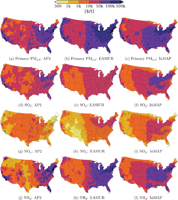
Figure 2. Marginal social costs for ground-level emissions for each US county by pollutant and by air quality model (in USD per tonne). Negative values are in shown in green.
Download figure:
Standard image High-resolution imageIn figures 3–6, we show the model inter-comparisons for each species for ground-level sources. Similar plots for elevated sources can be found in the supplemental information (figures S2–S5). All three RCMs provide damage estimates that are highly spatially resolved with respect to emissions location. Whereas some application scenarios will involve nationwide emissions changes, others may be focused on damages from emissions in one region of the country, perhaps a single state or even a single county. Therefore, it is worthwhile evaluating to what extent the three RCMs agree in terms of spatial patterns and county-by-county damage estimates. Here, we find that the level of agreement varies considerably by species according to the complexity of the associated chemistry, mirroring how some species are inherently more difficult to model than others, even for a CTM (figure S1). While all three RCMs estimate these social costs at high spatial resolution, the similarity of their answers depends on the species in question and the complexity of its atmospheric behavior. For ground-level primary PM2.5, the models have very similar values across all counties, with Pearson's correlation ranging from 0.73 to 0.81. For primary PM2.5, which is an inert species emitted directly in particulate form, concentrations are influenced only by differences in atmospheric transport and dilution. This is noted because it has been suggested that Gaussian dispersion modeling is not applicable at distances that exceed 100 km, yet we do not observe systematic biases in the AP2 estimates compared with the CTM-derived models. Consistent with the more complex chemistry, results for cost estimates for secondary pollutants are more variable on average and spatially, and the correlations of the secondary pollutants are lower: 0.54–0.73 for NH3, 0.35–0.49 for SO2 and 0.077–0.54 for NOx. The formation of secondary PM2.5 depends on how efficiently precursors are converted to secondary species. In the atmosphere, this typically depends on chemistry, deposition rates, sunlight and the availability of co-reactants, especially atmospheric oxidants and thermodynamic interactions between inorganic ions (Ansari and Pandis 1998, West et al 1999). Additionally, the impacts of secondary pollutants should also be more dependent on accurately predicting transport as chemical reactions can occur over long distances and thus expose populations further from the source. Thus, model selection has a larger role as the estimates of impacts depend on both the representation for long-range transport and chemical processes. Since 
 and
and  concentrations depend on each other, differences in the model predictions for one species will influence the others.
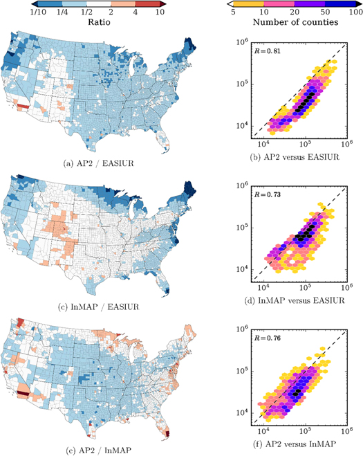
Figure 3. Comparison of marginal social costs from primary PM2.5 for ground-level emissions. Panels (a), (c) and (e) show the ratio of the social cost estimates for each county for each model pair. White counties indicate agreement within a factor of two. In panels (b), (d) and (f), the social costs of emissions (in USD per tonne) by county are plotted for each model pair to show the overall model agreement. R is the Pearson correlation coefficient.
Download figure:
Standard image High-resolution image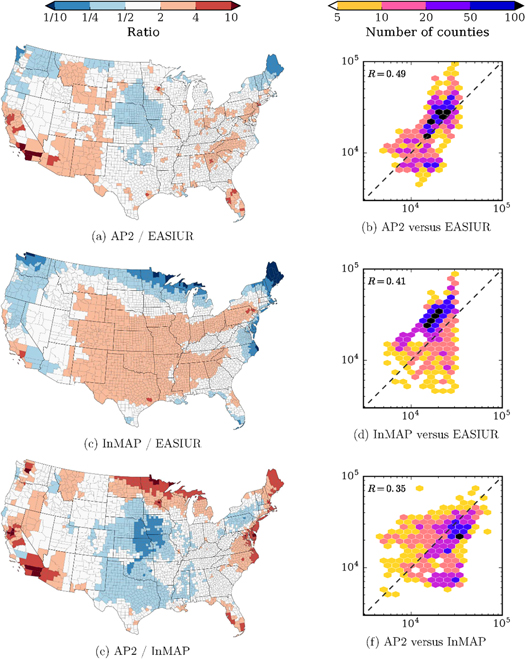
Figure 4. Comparison of marginal social costs of ground-level SO2 emissions. Panels (a), (c) and (e) show the ratio of the social cost estimates for each county for each model pair. White counties indicate agreement within a factor of two. In panels (b), (d) and (f), the social costs of emissions (in USD per tonne) by county are plotted for each model pair to show the overall model agreement. R is the Pearson correlation coefficient.
Download figure:
Standard image High-resolution image
Figure 5. Comparison of marginal social costs of ground-level NOx emissions. Panels (a), (c) and (e) show the ratio of the social cost estimates for each county for each model pair. White counties indicate agreement within a factor of two. In panels (b), (d) and (f), the social costs of emissions (in USD per tonne) by county are plotted for each model pair to show the overall model agreement. R is the Pearson correlation coefficient.
Download figure:
Standard image High-resolution image
Figure 6. Comparison of marginal social costs of ground-level NH3 emissions. Panels (a), (c) and (e) show the ratio of the social cost estimates for each county for each model pair. White counties indicate agreement within a factor of two. In panels (b), (d) and (f), the social costs of emissions (in USD per tonne) by county are plotted for each model pair to show the overall model agreement. R is the Pearson correlation coefficient.
Download figure:
Standard image High-resolution image
Finally, for the case of the impacts of SOA we are less confident that variability between current RCM estimates represents true prediction uncertainty than we are for inorganic PM2.5 species. This is because VOCs from different emissions sources can vary greatly in their SOA production efficiency and because the fundamental understanding of the formation of SOA from precursor VOCs is still rapidly evolving (Robinson et al 2007). At present, marginal social costs for VOC emissions are available from the InMAP and AP2 models, but the prediction of impacts from VOC emissions in RCMs is an area for future development. Specifically, RCMs that account for the fact that different sources have different mixes of VOCs and, therefore, different SOA to PM2.5 formation ratios and damage costs (Jathar et al 2014) would be desirable. When using SOA estimates from current RCMs, we recommend that users consider how the specific mix of VOC species that are relevant to their own scenarios compares with the anthropogenic average mixes implied within the RCMs. In cases where the VOC mixes are substantially different, chemical transport modeling with a more detailed treatment of VOC composition may be warranted.
5. Conclusion
The public health impacts of air pollution, mostly due to premature mortality caused by PM2.5 exposure, dominate the benefits analysis of most rules and regulations that target the energy and transportation sectors. Because evaluating these impacts using a state-of-the-science CTM can be challenging, several recent efforts have resulted in the development of RCMs that provide estimates of the marginal social costs stemming from a tonne of PM2.5 emissions and its precursors. In this letter we compare three datasets of air quality costs derived by RCMs: AP2, EASIUR and InMAP. We conclude that users can generally use marginal social costs reported by these models for decision and policy analysis in lieu of CTMs with only a modest loss of fidelity.
We show that the RCMs evaluated here can predict the nationwide distribution of PM2.5 concentrations with only a modest reduction in accuracy as compared with a CTM. Further, for analyzes at a national scale and over many sources, the differences in the air quality modeling approaches reviewed in this letter are less important for the aggregate social costs. Generally, for the evaluation of policies that are enacted at the national level, the total costs from all models are within a factor of two or three. Further, the differences in the social costs as a function of species emitted and source location are broadly similar between models and can be readily understood on the basis of the known atmospheric behavior of that species and the size of the downwind population exposed to PM2.5.
Additionally, the model estimates reviewed in this letter are derived from different air quality modeling approaches but with harmonized assumptions for the C–R function and the VSL. Hence, the range of the estimates presented here can be interpreted as a measure of the degree of uncertainty inherent in air quality modeling. Understanding why two CTMs produce different results is challenging as it is difficult to isolate all the factors that drive the differences. We face the same type of challenge when comparing the RCMs. Additionally, since each RCM takes a different approach to abstracting the physical and chemical processes for PM2.5 and the meteorology, it is even more challenging to isolate the factors. Thus, we focus on the substantive differences—the social costs—that are affected by the modeling choices made by each RCM. In general, the differences in air quality modeling introduced by and between the RCMs shown here are not large when viewed in the context of the other uncertainties in the damage estimates. These differences are small in comparison with other uncertainties involved in air quality decision-making, such as the C–R function (Fann et al 2016) and VSL (US EPA 2006). The differences in the damages are comparable to errors between CTMs as well as the errors between CTMs and observed ambient concentrations.
In some locations and for some pollutants, however, these differences can be more substantial; for example, it would be appropriate to investigate the range of benefit estimates for applications which are more geographically limited, and especially where NOx emissions are the dominant concern, such as the Marcellus shale development (Roy et al 2014) and replacing diesel engines for port power for shipping (Vaishnav et al 2016). Furthermore, there are cases where the RCM-derived social cost estimates should be applied with more caution, including when changes in emission occur for only a few days per year (e.g. Gilmore et al 2010) and when there is the potential for non-linearity or if the change in emissions is large enough to change the underlying chemical regimes (see Holt et al 2015).
While CTMs remain the gold standard for air quality simulation and should continue to be used in many regulatory settings, such as SIPs and regulatory impact assessments of major new rules, the ease of use of RCMs means that they can be used by a broad range of researchers and analysts. This may include initial scoping of new rules or regulations as well as decision-making in a large number of analyzes where the public health costs of air pollution are not routinely considered in a rigorous and explicit fashion. Because the social cost estimates from these RCMs are sensible and generally consistent and because they are far simpler to use than a CTM, we encourage researchers and analysts to use them in a broad range of applications when the public health impacts of air pollution may be important. Additionally, RCMs may open up more opportunities for assessing uncertainty. For example, in a CTM it is impractical to conduct a Monte Carlo type approach to capture the uncertainty in the emission inventories. As RCMs are less computationally expensive, these types of analyzes could be implemented. Finally, the successful development of RCMs for the US suggests that they might be developed and applied to other regions of the globe where air quality issues are more severe; however, this requires both suitable models and data.
Funding and acknowledgments
This publication was developed by funding from the Center for Air, Climate and Energy Solutions under Assistance Agreement no. RD83587301 awarded by the US EPA. It has not been formally reviewed by the US EPA. The views expressed in this document are solely those of the authors and do not necessarily reflect those of the Agency. The US EPA does not endorse any products or commercial services mentioned in this publication. JH acknowledges the US Department of Energy (grant no. EE0004397) and the US Department of Agriculture (grant nos 2011-68005-30411 and MIN-12-083).