


Abstract
The seasonal evolution of Arctic sea ice can be described by the timing of key dates of sea ice concentration (SIC) change during its annual retreat and advance cycle. Here, we use SICs from a satellite passive microwave climate data record to identify the sea ice dates of opening (DOO), retreat (DOR), advance (DOA), and closing (DOC) and the periods of time between these events. Regional variability in these key dates, periods, and sea ice melt onset and freeze-up dates for 12 Arctic regions during the melt seasons of 1979–2016 is investigated. We find statistically significant positive trends in the length of the melt season (outer ice-free period) for most of the eastern Arctic, the Bering Sea, and Hudson and Baffin Bays with trends as large as 11.9 d decade−1 observed in the Kara Sea. Trends in the DOR and DOA contribute to statistically significant increases in the length of the open water period for all regions within the Arctic Ocean ranging from 3.9 to 13.8 d decade−1. The length of the ice retreat period (DOR−DOO) ranges from 17.1 d in the Sea of Okhotsk to 41 d in the Greenland Sea. The length of the ice advance period (DOC−DOA) is generally much shorter and ranges from 17.9 to 25.3 d in the Sea of Okhotsk and Greenland Sea, respectively. Additionally, we derive the extent of the seasonal ice zone (SIZ) and find statistically significant negative trends (SIZ is shrinking) in the Sea of Okhotsk, Baffin Bay, Greenland Sea, and Barents Sea regions, which are geographically open to the oceans and influenced by reduced winter sea ice extent. Within regions of the Arctic Ocean, statistically significant positive trends indicate that the extent of the SIZ is expanding as Arctic summer sea ice declines.
Export citation and abstract BibTeX RIS

Original content from this work may be used under the terms of the Creative Commons Attribution 3.0 licence. Any further distribution of this work must maintain attribution to the author(s) and the title of the work, journal citation and DOI.
1. Introduction
Since late 1978, satellite passive microwave observations have been used to continuously monitor seasonal changes in sea ice concentration (SIC; the fractional coverage of sea ice within a grid cell) and sea ice extent (SIE; the summed area of grid cells where SIC ≥15%). During this period, SIE (Comiso et al 2008, Cavalieri and Parkinson 2012, Peng and Meier 2017), thickness (Lindsay and Schweiger 2015, Kwok 2018), age (Maslanik et al 2007), and volume (Kwok et al 2009) have declined dramatically. Arctic sea ice is now more susceptible to earlier melt onset (MO) (e.g. Mortin et al 2016, Bliss and Anderson 2018), more extensive summer retreat (e.g. Meier et al 2007, Cavalieri and Parkinson 2012), delayed autumn freeze-up (e.g. Markus et al 2009), and less extensive winter growth (e.g. Peng and Meier 2017, Onarheim et al 2018). The region is thus becoming more accessible, increasing opportunities for economic activity such as resource extraction, shipping, and tourism (ACIA 2004, IPCC 2014, Melillo et al 2014). Stakeholders can benefit from a set of indices to monitor and quantify changes in the seasonal evolution of Arctic sea ice; in particular, temporal changes in key dates during the annual sea ice retreat/advance cycle.
In this work, we present the first analysis of regional Arctic sea ice conditions using a full set of key dates of seasonal sea ice evolution including the dates of MO, opening, retreat, freeze onset (FO), advance, and closing for 12 Arctic sub-domains from the 37 year satellite passive microwave data record (1979–2016). From these dates, we also derive periods of sea ice loss, sea ice growth, the open water period, and the outer melt season. A conceptual diagram of the stages of annual sea ice evolution at a location is shown in figure 1, with acronyms defined in table 1. This work expands upon the study by Peng et al (2018), which examines the pan-Arctic seasonal evolution of the sea ice retreat/advance cycle dates and periods. Here we focus on the regional variability of seasonal dates and periods for domains defined in figure 2 and examine change in the seasonal ice zone (SIZ; the area in which sea ice melts out after the winter maximum sea ice extent) to quantify the annual extent of summer sea ice retreat.
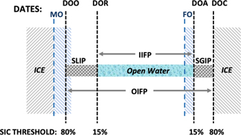
Figure 1. Conceptual diagram of sea ice seasonal evolution from spring/summer retreat (left) through fall/winter advance (right). Acronyms for the dates and periods between dates are defined in table 1. Black vertical dashed lines show dates of opening/closing and retreat/advance with corresponding sea ice concentration (SIC) thresholds at bottom. Horizontal arrows span the outer and inner ice-free periods. Blue hatched areas indicate windows during which melt onset (MO) dates can occur and freeze onset (FO) dates of the perennial sea ice cover before sea ice advance begins. See text for more details.
Download figure:
Standard image High-resolution imageTable 1. Acronyms and definitions of dates and periods derived from dates.
| Acronym | Expansion | Definition |
|---|---|---|
| MO | Melt onset | Date of the onset of snow and sea ice melting |
| DOO | Day of opening | Last day SIC drops below 80% before the summer minimum |
| DOR | Day of retreat | Last day SIC drops below 15% before the summer minimum |
| DOA | Day of advance | First day SIC increases above 15% following the final summer minimum |
| DOC | Day of closing | First day SIC increases above 80% following the final summer minimum |
| SLIP | Seasonal loss of ice period | Defined as DOR−DOO |
| SGIP | Seasonal gain of ice period | Defined as DOC−DOA |
| IIFP | Inner ice-free period | Defined as DOA−DOR; the open water period |
| OIFP | Outer ice-free period | Defined as DOC−DOO |
| FO | Freeze onset | The freeze-up date of perennial sea ice after the summer sea ice extent minimum |
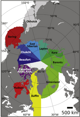
Figure 2. Regions of the Arctic. The hatched region is omitted from the regional analysis as described in text.
Download figure:
Standard image High-resolution image2. Data and methods
2.1. Melt season dates and periods
The dates of sea ice opening, retreat, advance, and closing are identified from the time series of daily SIC from the NOAA/NSIDC SIC climate data record (CDR) v3r01 (Meier et al 2017) which are derived from NASA's scanning multichannel microwave radiometer (SMMR), and the series of defense meteorological satellite program special sensor microwave imager (SSM/I) and special sensor microwave imager/sounder (SSMIS) sensors. We use SICs from the 25 km resolution 'Goddard Merged' parameter in the CDR product (Peng et al 2013), which is produced by merging SICs from the NASA Team (Cavalieri et al 1984) and Bootstrap (Comiso 1995) algorithms. In this work, we define the ice year from 1 March through 28 February of the following year to capture the initiation of the melt season (beginning with MO) through the subsequent freeze-up period and name the seasonal cycle for the year in which the melt season occurs (e.g. the 2016 seasonal cycle is obtained using data from 1 March 2016–28 February 2017).
A 7 d boxcar running mean is applied to the time series of daily SIC at each grid pixel to eliminate some of the noise due to dynamic ice transport over short timescales (Comiso 2002), which is not uncommon during sea ice retreat (Steele et al 2015). The smoothed time series of daily SIC for the ice year 1 March through 28 February of the following year are used to derive the dates and periods of seasonal sea ice evolution. The 15% ice concentration threshold is commonly used to discriminate between sea ice and open ocean covered grid cells, while the 80% DOO threshold typically marks the date when SIC declines toward the annual minimum (Markus et al 2009, Steele et al 2015) and is the upper SIC threshold used by the US National Ice Center to define the marginal ice zone boundary (Strong and Rigor 2013). The decrease in SIC from 80% to 15% is frequently nonlinear as the SIC can vary from day-to-day due to wind advection (Steele et al 2015); therefore, we take the last day that SIC drops below the thresholds to obtain the DOO and DOR (table 1). Similarly, we take the first days that SIC increases above the thresholds to obtain the DOA and DOC (table 1) identifying when the ice first returns which may be more valuable to stakeholders. The DOO, DOR, DOA, and DOC for each year are determined for grid cells where the mean March SIC ≥ 90%. A DOA (DOC) is only identified at grid cells where a valid DOR (DOO) was identified prior to the summer sea ice minimum. The resulting data set of seasonal dates and periods used in this analysis including the MO and FO dates described below can be obtained from Steele et al (2019).
2.2. Melt and FO dates
Several methods to detect sea ice MO and FO from passive microwave satellite data exist; thus, there are several ways to define the dates of MO and FO (e.g. Bliss et al 2017). Here, we use three dates of MO and two FO dates. MO dates representing the earliest date when the snow and/or sea ice surface become wet due to melting are from the Drobot and Anderson (2001) Advanced Horizontal Range Algorithm (hereafter AHRA MO; Anderson et al 2014, Bliss and Anderson 2018). We also compute an early MO date (EMO), continuous MO date (CMO), early FO date (EFO), and continuous FO date (CFO) using the Passive Microwave (PMW) algorithm developed by Markus et al (2009). The timing of AHRA MO dates and the EMO and CMO dates are significantly different due to differences in passive microwave channel sensitivity and algorithm differences as described by Bliss et al (2017). Similar to EMO and CMO dates, the EFO corresponds to the first date that freeze-up occurs and the CFO indicates the date on which freezing conditions persist until the following melt season begins. In cases when the PMW algorithm cannot identify a clear melting or freezing signal, the algorithm identifies MO dates when SIC from the NASA Team algorithm drops below 80% for the last time before the area becomes seasonally ice-free and identifies FO dates when NASA Team SIC increases to 80% for the first time after the sea ice minimum. Thus, in some cases (primarily in the SIZ) the CMO is equivalent to the DOO. For this work, we modified the PMW algorithm by using the CDR 'Goddard Merged' SIC instead of the NASA Team SIC, for consistency with other dates used in this study.
2.3. Methodology for regional statistics
In order to calculate consistent statistics, we first mask all dates and periods to locations that have a valid DOR (figure S1 is available online at stacks.iop.org/ERL/14/045003/mmedia; see also Peng et al 2018) excluding the EFO and CFO dates. Regional statistics for EFO and CFO dates are calculated for the surviving summer sea ice extent (i.e. poleward of the northern extent of grid cells where a valid DOR was found). In some cases, the SIE has not yet reached its annual maximum by the end of our defined ice year on 28 February; therefore, DOA and DOC along the southern ice periphery where ice typically forms in late winter may not be identified and are ignored when statistics are calculated. Regional statistics including means, standard deviations, and decadal trends are calculated from masked dates and periods for 12 Arctic sub-regions (figure 2). Sea ice does not frequently retreat within the area north of Greenland and the Canadian Arctic Archipelago region (hatched area in figure 2) during the study period (figure S2); thus, this area is omitted from the analysis. The regional boundaries in this work are similar to those used in many other studies (e.g. Meier et al 2007, Peng and Meier 2017, Bliss and Anderson 2018). It should be noted that local forcing on the dates at scales smaller than the regions used here warrant further investigation (e.g. Steele et al 2015). Trends are calculated using a linear least squares regression approach.
2.4. Seasonal ice zone
To determine the extent of the SIZ, we create a binary grid that assigns a value of 1 to grid cells that (1) have a valid DOR, (2) have a March monthly SIC ≥ 15%, and (3) have a SIC < 15% at the minimum SIE. The geographic areas (in km2) of grid cells where the above three criteria are met are summed yielding the annual SIZ extent. To create a consistent time series of March SIE, we assume that the region between 84.5 °N (the SMMR pole hole extent) and 89.18 °N (the SSMIS pole hole extent) is effectively sea ice covered during March in all years of the study period. In this work, surviving summer sea ice refers to the sea ice (SIC ≥ 15%) remaining at the annual extent minimum (i.e. sea ice where no DOR is identified) including all area between the SMMR and SSMIS pole hole extents that we assume to be ice-covered. The surviving summer sea ice is analogous to the perennial ice extent (Comiso 2002) that is primarily composed of multi-year ice floes and some seasonal ice that can age and thicken during the subsequent winter.
3. Results
3.1. SIZ extent
Figure S1 illustrates the SIZ extent for each year during the study period (dark blue) and the extent of the surviving sea ice at the end of the melt season during the given year (light blue). The size of the SIZ extent depends on both the winter maximum SIE and the extent of sea ice retreat during the summer; thus, an increase (decrease) in the extent of the SIZ could be related to either decreases (increases) in summer SIE or increases (decreases) in winter SIE. Over the 1979–2016 study period, the SIZ extent increases to over 10 × 106 km2 after 1990, although the historical minimum SIZ extent from the continuous satellite record (7.95 × 10⁶ km2) occurs in 1996—the record high SIE minimum year (Serreze and Stroeve 2015). The SIZ extent reached a maximum of 12.23 × 10⁶ km2 in 2012, the current record lowest sea ice minimum (Parkinson and Comiso 2013, NSIDC 2017). Interestingly, 2016 and 2007 are tied for second lowest sea ice minimum (NSIDC 2017); however, more extensive winter SIE in the St. Lawrence Gulf and Baffin Bay regions (figure S1) contribute to a larger SIZ extent in 2008 despite this year holding the 6th place record for minimum SIE (NSIDC 2017).
At the regional scale, in most peripheral regions that are geographically open to the south (i.e. the Okhotsk, Baffin, Greenland, and Barents regions), March SIE is variable from year to year with statistically significant trends ranging from −0.6 × 10⁵ km2 to −1.02 × 10⁵ km2 per decade (figure 3); the exception is the Bering region, which has no significant trend. The remaining regions are either geographically landlocked like Hudson Bay or located within the central Arctic and away from the ice periphery (i.e. the Kara, Laptev, E Siberian, Chukchi, Beaufort, and Canadian Arctic regions). Thus, these regions are entirely ice covered during March in all years excluding March 2008 in the Kara Sea when small ice-free areas were present (∼5191 km2 in total).
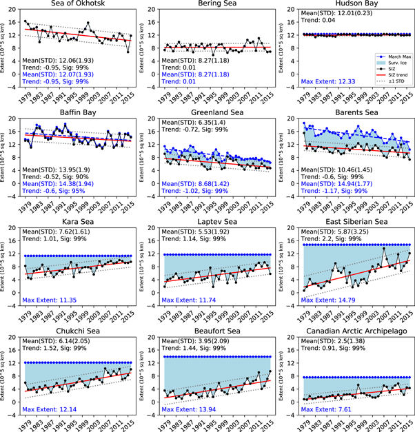
Figure 3. Regional time series and statistics for March monthly sea ice extent (SIE) in dark blue and seasonal ice zone (SIZ) extent in black for 1979–2016. The light blue shaded area is representative of the surviving SIE at the end of the melt season. The least squares linear trend in SIZ extent is shown in red with dotted lines to indicate ±1 standard deviation. The confidence level for statistically significant trends is noted.
Download figure:
Standard image High-resolution imageIn the Okhotsk, Baffin, Greenland, and Barents regions, trends in SIZ extent and March SIE are negative, indicating that some of the trend in SIZ extent is driven by the reduction in winter SIE. In regions that are fully sea ice covered in March (i.e. no inter-annual variability and no trend in March SIE) excluding Hudson Bay, the SIZ extent is increasing and has statistically significant positive trends ranging from 0.91 × 10⁵ km2 per decade in the Canadian Arctic to 2.2 × 10⁵ km2 per decade in the E. Siberian region (figure 3). The filled area between the March SIE and SIZ extent in figure 3 corresponds to the extent of surviving sea ice at the end of the melt season (i.e. the perennial sea ice) within the region (figure S1). Given the relatively small amount of surviving sea ice observed in recent years in the Kara and Chukchi regions, if we assume that positive trends in SIZ extent persist, a simple extrapolation of the trends suggests that these two regions are most at risk of becoming ice-free during the summer within the next two decades (figure 3; Peng and Meier 2017, Onarheim et al 2018).
These results expand on an analysis by Kinnard et al (2008) who found a gradual expansion of the SIZ since 1870 with a marked acceleration over the satellite era. The seasonality of Arctic sea ice has also been quantified by Haine and Martin (2017) using a metric to describe the annual range in SIE (winter max–summer min). They show that the seasonality of Arctic sea ice is increasing, driven largely by the record low summer SIE observed in recent years, which is also evident in our SIZ extent for Arctic Ocean regions (figure 3). Countering the growth of the SIZ due to increasing summer retreat, continued reductions in winter SIE would contribute to future reductions in SIZ extent (i.e. a smaller winter SIE means there is less SIE available to be melted during the subsequent melt season) as is seen currently in the open, peripheral sea ice regions (figure 3).
3.2. Seasonal evolution
The seasonal evolution of the sea ice retreat/advance cycle over the years 1979–2016 is shown for three representative regions—the Beaufort, Barents, and Hudson Bay regions in figures 5–7, respectively. Data for the eight remaining regions and for all Northern Hemisphere sea ice are shown in figures S3–S12. In all regions, the AHRA MO date occurs earliest in the year, signaling the initial MO of the snow and/or sea ice cover and followed by the EMO and CMO dates. The relative lengths of the SLIP, IIFP, and SGIP vary from year to year. The mean annual EFO and CMO dates are much earlier than the mean DOA and the onset of the SGIP period (e.g. figures 5, 6) since they indicate the FO dates of the surviving sea ice adjacent to and north of the SIZ.
The Beaufort Sea is an example of a region that is fully ice-covered in winter, with an increasing trend in the size of the SIZ each melt season (figures 4, 5). The length of the IIFP is variable from year to year ranging from a minimum of 16.3 d in 1985 to a maximum of 131.1 d in 1998. The length of the SLIP ranges from 17.5 to 52.7 d and is consistently longer than the autumn SGIP, which ranges from 7.4 to 28.7 d. The melt season generally begins in mid-May with the AHRA MO date indicating the initial MO, with the MO period further developing through May and June. Following the retreat period, FO of the surviving sea ice cover generally begins in late August and early September, before sea ice advance in the southern extents of the regions begins near the beginning of October.
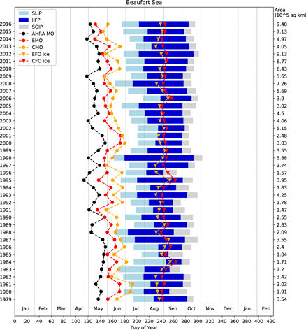
Figure 4. Mean annual evolution of the sea ice melt season for the Beaufort Sea region (1979–2016). Colors for the shaded bars define the mean seasonal loss of ice period (SLIP), inner ice-free period (IIFP), and seasonal growth of ice period (SGIP). The full span of the shaded bars defines the outer ice-free period (OIFP). Curves noted with filled circles show annual mean melt onset (MO) dates including the AHRA MO, early melt onset (EMO) and continuous melt onset (CMO) dates. Curves noted with filled triangles show the annual mean freeze onset (FO) dates of surviving summer sea ice within the region and adjacent to the seasonal ice zone (SIZ) including the early freeze onset (EFO) and continuous freeze onset (CFO) dates. Areas noted on right axis give the area of grid cells with an observed date of retreat (DOR) for the region.
Download figure:
Standard image High-resolution image
Figure 5. Same as figure 4 for the Barents Sea region.
Download figure:
Standard image High-resolution imageThe Barents Sea (figure 5) is representative of an open, peripheral ice region (described in section 3.1) where both the winter SIE and summer retreat extent vary. In this region, the length of the IIFP is longer than that for the Beaufort Sea ranging from 76.6 d in 1992 to 162.3 d in 2006. Like the Beaufort Sea region, the SLIP (ranging from 19.9 to 39.6 d) in the Barents Sea is generally longer than the SGIP (ranging from 8.8 to 34.0 d). There is also more spread between MO dates computed using AHRA versus EMO and CMO algorithms, possibly due to the larger presence of first-year ice in this region where the PMW algorithm frequently uses a SIC threshold to identify a MO date; thus, producing a delayed EMO and CMO date relative to the AHRA MO date (Bliss et al 2017).
The Hudson Bay is unique in that it is landlocked and is fully ice-covered in the winter with near complete retreat of sea ice each year (figure 6). Similar to the Barents Sea region, Hudson Bay has a longer IIFP than the Beaufort Sea ranging from 99.8 d in 1986 to 166.3 d in 2010; however, the periods and dates in this region are less variable from year to year than both the Barents and Beaufort regions (figures 5, 6). This region occupies a lower latitude band and is influenced more by warmer continental air masses during the summer than the other regions. Additionally, the dominant ice type in Hudson Bay is seasonal ice (e.g. figures 3, 4), which is more susceptible to full retreat each year without the increased variability of the dates and periods observed in Arctic Ocean regions with more perennial ice extent (compare also figures S3, S4).
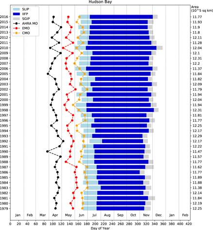
Figure 6. Same as figure 4 for the Hudson Bay region. Early freeze onset (EFO) and continuous freeze onset (CFO) curves are omitted from this plot due to the lack of surviving sea ice. See text for more details.
Download figure:
Standard image High-resolution image3.3. Regional statistics of dates
Decadal trends indicate that the AHRA MO is occurring earlier in the year for most regions within the Arctic Ocean (table 2; see table S1 for regional means and standard deviations). Significant AHRA MO trends <−5.0 d decade−1 are observed in the Laptev, E Siberian, Kara, and Barents regions. Statistically significant negative trends in CMO date are present for all regions excluding the Okhotsk, Bering, Laptev, and E. Siberian regions, with the strongest trend of −5.6 d decade−1 found in the Beaufort Sea. Earlier MO dates (negative trends) are often associated with increased downwelling longwave radiation in the spring due to enhanced atmospheric moisture and cloud cover (Mortin et al 2016); however, inter-annual variability in MO timing is generally large at the regional scale with mean standard deviations >12 d for some regions (table S1) due to variability in spring weather conditions (e.g. Drobot and Anderson 2001). For regions where some sea ice survives the summer melting season, no significant trends in the EFO or CFO dates were found. This is likely related to the cooling of surface air temperatures over the surviving sea ice as the sun angle decreases into early September, the mean FO date in these regions (table S1) (Perovich et al 2007, Markus et al 2009).
Table 2. Regional decadal trendsa (days decade−1) of dates.
| Region | AHRA MO | EMO | CMO | DOO | DOR | DOA | DOC | EFO Ice | CFO Ice |
|---|---|---|---|---|---|---|---|---|---|
| Okhotsk | −0.2 | 1.4 | 1.1 | −0.1 | −0.6 | −0.6 | 0.1 | N/A | N/A |
| Bering | 0.9 | −1.3 | −1.5 | −1.2 | −2.2 | 3.7 | 3.6 | N/A | N/A |
| Hudson | −1.7 | −4.0 | −3.3 | −4.4 | −6.5 | 5.1 | 4.2 | N/A | N/A |
| Baffin | −1.7 | −2.2 | −3.0 | −4.2 | −5.5 | 3.5 | 3.1 | N/A | N/A |
| Greenland | 2.4 | −0.3 | −2.5 | −1.0 | −1.8 | −0.2 | −1.6 | 1.2 | 1.2 |
| Barents | −6.1 | −3.1 | −5.0 | −3.6 | −5.6 | 6.1 | 4.9 | 1.5 | 0.3 |
| Kara | −6.0 | −4.2 | −2.8 | −6.7 | −7.8 | 6.0 | 5.3 | 1.3 | −0.1 |
| Laptev | −5.4 | −1.7 | −1.3 | −2.4 | −4.2 | 5.4 | 4.4 | 0.0 | −0.4 |
| E. Siberian | −7.5 | −0.3 | 0.5 | −2.0 | −4.9 | 6.1 | 5.3 | 0.5 | 0.1 |
| Chukchi | −1.7 | −1.7 | −3.6 | 0.5 | 0.0 | 3.9 | 2.2 | 0.2 | −0.3 |
| Beaufort | −3.1 | −4.4 | −5.6 | −0.2 | −2.1 | 5.1 | 3.1 | 0.2 | −0.3 |
| Canadian Arctic | −1.7 | −1.7 | −3.2 | −0.4 | −3.5 | 1.7 | 1.0 | 1.4 | 1.4 |
aSignificance level of trends are noted as follows: italic = 90%, bold = 95%, italic and bold = 99%.
Statistically significant decadal trends in the DOO occur in the Hudson and Baffin Bays and in the eastern Arctic including: the Barents, Kara, and Laptev regions, while in other regions, non-significant trends in the DOO are near 0 and generally negative except in the Chukchi Sea (table 2). In an analysis for the Beaufort Sea, the DOO was shown to be sensitive to local forcing such as winds with stronger trends observed in DOR than in DOO (Steele et al 2015). The lack of significant trends in DOO for some of our regions suggests that the domains may be too large to observe the effects of local forcing. Our results show trends in the DOR are generally stronger and significant in more regions than for the DOO, consistent with the previous study. Significant trends in the DOR < −5 d decade−1 are present in the Hudson, Baffin, Barents, and Kara regions. Positive trends in the DOA and DOC indicate that sea ice growth after the summer minimum is being delayed over the satellite era. Statistically significant trends in the DOA are present in all regions excluding the Okhotsk and Greenland regions. Similarly, significant trends in the DOC are positive for most Arctic regions excluding the Okhotsk, Greenland, and Canadian Arctic regions. Trends toward later DOA and DOC are consistent with the effects of earlier MO and DOR that increase the amount of solar radiation absorbed by the ocean and increase sea surface temperatures which then delay freeze-up (Steele and Dickinson 2016).
3.4. Regional statistics of periods
The SLIP is on average longer than the SGIP in all regions excluding the Okhotsk region (figures 7(a), (b)), ranging from 26 to 29.3 d in the eastern Arctic regions and ≥30 d in the Beaufort, Canadian Arctic, and Greenland regions. The SGIP is longest in the Greenland, Barents, and the Canadian Arctic regions where SGIP exceeds 20 d. Shorter SGIP (10.3 to 13.1 d) occurs in the Kara, Laptev, E. Siberian, and Chukchi regions relative to the Bering and Okhotsk regions (15 and 17.9 d), which is likely related to the comparatively fast freeze-up of seasonal ice areas at higher latitudes. The mean IIFP is much longer in the peripheral Arctic regions, exceeding 200 d in both the Bering and Okhotsk regions and exceeding 110 d in the Barents, Hudson and Baffin regions (figure 7(c)). Shorter IIFP occurs in the E. Siberian, Canadian Arctic, Laptev, and Beaufort regions, ranging from 47.1 to 58.6 d where the DOR occurs relatively late in the melt season and DOA occurs shortly after. A regional pattern similar to the IIFP is found for the mean OIFP, with the greatest OIFP of 252.2 d found in the Okhotsk region (figure 7(d)), reflecting the short sea ice season in this region (Parkinson 2014). There is high inter-annual variability in the lengths of the IIFP and OIFP with the largest standard deviations (∼20 d) in the Kara and Barents regions (figures 7(g), (h)) where the ice is sensitive to the transport of ocean heat from the Atlantic (Årthun et al 2012) and warm, humid air from the south (e.g. Boisvert et al 2016, Mortin et al 2016).

Figure 7. Regional statistics for the (left to right) SLIP, SGIP, IIFP, and OIFP including: (top row) mean length, (middle row) standard deviation, and (bottom row) decadal trend for 1979–2016. Significance level of the regional trend (bottom row) is noted by text color with black text indicating the trend is not significant. Statistics are also summarized in tables S2, S3.
Download figure:
Standard image High-resolution image
Strong positive trends in length of the IIFP are present in all regions except the Sea of Okhotsk and the Greenland Sea (figure 7(k)). Negative trends in the DOR (earlier retreat) combined with positive trends in the DOA (later advance) (table 2) contribute to the significant lengthening of the IIFP by more than 9 d decade−1 in all eastern Arctic Ocean regions and the Hudson and Baffin Bay regions (figure 7(k)). These results are consistent with the lengthening of the open water period reported by several other studies (e.g. Markus et al 2009, Parkinson 2014). Similar patterns in regional trends are found for the OIFP (figure 7(l)). However, trends are slightly smaller for all regions except in the Laptev Sea and not statistically significant in the Chukchi, Beaufort, and Canadian Arctic regions. For most regions, the SLIP period is becoming slightly shorter (figure 7(i)), which may be related to the reduction in the frequency of multiple ice edge loitering events noted by Steele and Ermold (2015), i.e. the ice pack is more quickly transitioning from full ice cover to open water each summer. The SGIP period is also shortening slightly for some regions, where statistically significant negative trends of ∼1–2 d decade−1 exist for the Hudson, Greenland, Laptev, E. Siberian, Chukchi, and Beaufort regions. This is a bit surprising given the lengthening IIFP, which allows more ocean warming. However, Onarheim et al (2018) note an increase in the frequency of rapid ice growth events in recent years with record low SIE minima, which may be due to strong ocean salinity stratification, limiting vertical mixing and allowing the surface layer to cool quickly. The combination of extensive summer retreat, delayed freeze-up, and the resulting rapid advance of sea ice could contribute to the observed SGIP shortening in the Beaufort, Chukchi, E. Siberian, and Laptev regions.
Previous investigations of Arctic sea ice dates of retreat (DOR) and advance (DOA) reported a strong inverse relationship (Stammerjohn et al 2012, Stroeve et al 2016), that is largely attributed to the seasonal ice-albedo feedback mechanism where earlier spring retreat leads to increased ocean heat uptake and warmer sea surface temperatures during the summer (Steele and Dickinson 2016). Further, Stroeve et al (2016) found that weaker correlations exist where effects such as strong winds, ocean currents and heat transport, and river discharge may impact the DOA more so than thermodynamic mechanisms related to ice-albedo feedback. Thus, dynamic effects limit the predictability of DOA timing based on the timing of the DOR in regions where the DOA is strongly controlled by local factors. Other studies also highlight the importance of local effects on sea ice retreat such as Steele et al (2015) who compared the DOO and DOR in the Beaufort Sea and demonstrated the local predictive effects of easterly wind anomalies in the E. Beaufort Sea contributing to earlier DOO and Serreze et al (2016) who demonstrated that ocean heat transport through Bering Strait explains 68% of variance in the DOR and 67% of the variance in the DOA for the southern Chukchi Sea. The full set of seasonal sea ice dates and periods can be used for future examination of the interrelationship between the dates and local scale forcing for any sub-Arctic domain.
4. Summary and conclusions
The work presented here provides a new baseline statistical analysis of regional change in Arctic sea ice seasonal evolution from satellite passive microwave data over the years 1979–2016 by identifying key stages of the seasonal sea ice retreat/advance cycle. We show that the SIZ extent is increasing in regions within the Arctic Ocean largely due to the increased sensitivity of the ice to summer melting as evidenced by the expansion of poleward retreating sea ice; however, decreases in winter SIE as seen in the Okhotsk, Baffin, Greenland, and Barents regions will begin to impact SIZ extent to a larger degree. Trends in the SIZ extent suggest that the Kara and Chukchi Seas are next to transition towards seasonally ice-free conditions, becoming more similar to peripheral regions such as the Okhotsk, Baffin, Greenland, and Barents regions. Trends in the DOR and DOA contribute to significant increases in the length of the IIFP ranging from 3.9 to 13.8 d decade−1, which increases the amount of solar energy absorbed by the ice-ocean system during the melt season. Further investigation is needed to study the local forcing on the dates and periods at regional scales smaller than those reported here.
Acknowledgments
The authors declare no conflicts of interest. This work was funded by NASA grant NNX16AK43G (all authors) and NSF grant OPP-1751363 (M Steele). The authors thank J A Miller for providing the modified PMW algorithm melt and freeze onset dates. The new data set used in this analysis is distributed by the National Snow and Ice Data Center Distributed Active Archive Center. See Steele et al (2019) to obtain the data. The authors thank two anonymous reviewers whose feedback improved the clarity and presentation of this work.