

Abstract
The uncertainties in sea ice extent (total area covered by sea ice with concentration >15%) derived from passive microwave sensors are assessed in two ways. Absolute uncertainty (accuracy) is evaluated based on the comparison of the extent between several products. There are clear biases between the extent from the different products that are of the order of 500 000 to 1 × 10⁶ km2 depending on the season and hemisphere. These biases are due to differences in the algorithm sensitivity to ice edge conditions and the spatial resolution of different sensors. Relative uncertainty is assessed by examining extents from the National Snow and Ice Data Center Sea Ice Index product. The largest source of uncertainty, ∼100 000 km2, is between near-real-time and final products due to different input source data and different processing and quality control. For consistent processing, the uncertainty is assessed using different input source data and by varying concentration algorithm parameters. This yields a relative uncertainty of 30 000–70 000 km2. The Arctic minimum extent uncertainty is ∼40 000 km2. Uncertainties in comparing with earlier parts of the record may be higher due to sensor transitions. For the first time, this study provides a quantitative estimate of sea ice extent uncertainty.
Export citation and abstract BibTeX RIS

Original content from this work may be used under the terms of the Creative Commons Attribution 3.0 licence. Any further distribution of this work must maintain attribution to the author(s) and the title of the work, journal citation and DOI.
1. Introduction
Sea ice extent is a widely used polar climate indicator and the significant decreasing trend in Arctic summer sea ice extent over the past forty years is one of the most iconic indicators of climate change. Sea ice extent is defined as the total surface area covered by sea ice above a certain concentration threshold (usually 15%). It has most commonly been derived from passive microwave imagery. The advantage of passive microwave data is that they provide all-sky (including darkness and cloudy conditions) capability; that and the sensor properties (i.e. a wide swath) allow complete daily coverage. In addition, a consistent series of sensors since the end of 1978 have now provided a nearly-complete high-quality 40-year record of sea ice extent.
Passive microwave brightness temperature data are used to derive sea ice concentration (fractional ice cover) based on empirically derived algorithms, typically as gridded daily average fields. The extent is then computed by summing the area of all grid cells with a concentration above the defined threshold.
Several different algorithms and products have been developed based on the passive microwave record. Over the years there have been numerous validation studies conducted to estimate the uncertainties of the concentration fields (e.g. Ivanova et al 2015) as well as ice edge position (e.g. Partington 2000). These have been based on comparison with higher spatial resolution visible, infrared, or synthetic-aperture radar data on satellite, airborne, and occasionally ship-borne platforms. However, these studies have been conducted on a limited set of validation data, usually over small regions and a relatively short period of time. Trends from sea ice extent from different products have been intercompared (e.g. Comiso et al 2017). However, to date there has not been an attempt to quantify the uncertainty in daily or monthly total sea ice extent estimates from passive microwave instruments.
Here we assess extent uncertainty in two ways. First, we compare several extent products and determine the range of the estimates. This provides an indication of the absolute uncertainty (accuracy) of the extent; in other words, it provides a range of how much total sea ice there is. Second, we estimate the relative uncertainty (precision) of one extent product, the National Snow and Ice Data Center (NSIDC) Sea Ice Index (SII; Fetterer et al 2017), to determine the consistency of the estimates over time; this yields the uncertainty of any given estimate (e.g. for a day or a month) relative to other times from the same product.
2. Background
This study uses the multichannel passive microwave satellite record, which spans from late 1978 through to the present. Further information on the instruments is provided in the supplementary materials available online at stacks.iop.org/ERL/14/035005/mmedia; here we simply list (table 1) the primary sensors and platforms discussed in this paper. The sensors retrieve the parameter 'brightness temperature', Tb, which is an indication of the emitted energy by a surface. For a given surface with a given physical temperature, Tb values vary with frequency and polarization.
Table 1. Passive microwave sensors and satellites used for long-term records of sea ice concentration and extent, as of August 2018.
| Sensor | Satellite(s) | Years of operation for sea ice products |
|---|---|---|
| Scanning multichannel microwave radiometer (SMMR) | NASA Nimbus-7 | Oct 1978–Aug 1987 |
| Special sensor microwave imager (SSMI) | DMSP F8, F11, F13 | Jul 1987–Dec 2007 |
| Special sensor microwave imager and sounder (SSMIS) | DMSP F16, F17, F18 | Jan 2007–present |
| Advanced microwave scanning radiometer for EOS (AMSR-E) | NASA Earth Observing System (EOS) Aqua | May 2002–Oct 2011 |
| Advanced microwave scanning radiometer 2 (AMSR2) | JAXA Global Change Observation Mission for Water (GCOM-W) | Jul 2012–present |
Several algorithms have been developed to derive sea ice concentration (fractional coverage of ice) from Tb via empirically derived algorithms. The different algorithms use different combinations of frequency and polarization channels, but generally share the common approach of finding coefficients (called 'tiepoints') for pure surface types (100% ice, 100% water) and interpolating between these to find the concentration that corresponds to a set of Tb values. Post-processing is typically conducted to remove spurious sea ice retrievals due to weather and coastal effects (mixed land/ocean grid cells) and to fill in missing data with spatial and/or temporal interpolation. More details on concentration algorithms and associated references are provided in the supplementary material.
In this study, we employ the commonly used 15% concentration threshold to define the edge. The original rationale for this threshold comes from early validation studies that found the 15% concentration contour agreed best with the 'true' ice edge in high-resolution airborne or satellite data (e.g. Cavalieri et al 1991). Due to satellite orbit characteristics, the passive microwave instruments have a gap ('pole hole') in coverage near the pole; the size of the gap has varied between different sensors. The gap for all sensors is assumed to be ice-covered (>15%) and the pole hole area is included in the extent total.
Another practical reason for the 15% threshold is that most algorithms apply a post-processing 'weather filter' to remove erroneous ice due to emission from the atmospheric and wind roughening of the ocean surface. This filter is generally a 'gradient ratio' (GR)—a normalized difference between two frequencies. For sea ice, two GRs are commonly used: Tbs from the vertical polarizations of (1) 37 GHz and 19 GHz and (2) 22 GHz and 19 GHz frequencies. The relevance for the ice edge is that while the goal is to remove weather artifacts, in practice it removes some low-concentration ice. Using the 15% threshold avoids having the GR filter affect the extent estimates. The GR filter and its influence on extent are examined in more detail in section 4.
Subsequent comparisons (e.g. Partington 2000) have found that the representativeness of the 15% contour to define the ice edge can vary considerably depending on the character of the ice near the edge. The sea ice edge is not necessarily a sharp boundary, rather it is often a mélange of ice floes of varying thickness and sizes intermixed with open water. The sensitivity of passive microwave imagery to such thin ice and small floes is variable. The concentration retrieved may fall below the 15% threshold even when substantial (>15%) ice remains, depending on the aggregate effect of the concentration, size of floes, presence of melt ponds, and ice thickness of the observed region.
The ice edge determination, and hence an extent estimate, are also dependent to some degree on the spatial resolution of the sensor and, because resolution varies with frequency, the frequencies used by a given algorithm. Lower resolution may lead to a 'smearing out' of the ice edge, leading to an overestimate of the edge. On the other hand, the smearing may compensate for the limited performance in thin and melting ice, which is most prevalent near the ice edge. This has important ramifications when interpreting differences in extents from different sea ice products.
Here we evaluate extent uncertainty in two ways: (1) absolute uncertainty via comparison of extents from several different products, and (2) relative uncertainty by comparing extent variability with different inputs and processing. The primary extent estimates are from the NSIDC SII version 3 (Fetterer et al 2017, http://nsidc.org/data/seaice_index/). The SII extents are derived from two sources of gridded sea ice concentration fields. For recent data, near-real-time (NRT) sea ice concentrations from the NASA team algorithm (Maslanik and Stroeve 1999), processed at NSIDC, are employed. The NRT fields are replaced by 'final' concentration fields when data are processed by NASA Goddard (also using the NASA team algorithm) (Cavalieri et al 1996).
3. Absolute uncertainty
The most basic questions concerning sea ice extent are just how much of the ocean surface is covered by ice and how well can we measure it? In other words, what is the accuracy, or absolute uncertainty, of the estimates compared to the 'true' extent? While conceptually straightforward, determining the accuracy of sea ice extent estimates is difficult because there is no polar-wide, independent, accurate, and consistent data product with which to compare the passive microwave estimates. Here we calculate a range of extents based on the different products to represent an estimate of absolute uncertainty.
3.1. Approach
The approach we use is to simply look at an ensemble of estimates from different products. We assume that no passive microwave product is perfect and no estimate will be 'correct'. However, by comparing extent estimates of several different products, we can use the variation between the estimates to provide a range of extent values into which the true extent is likely to fall. Of course, this is not necessarily the case: all of the estimates may be biased high or low. But the ensemble of extent values at least provides a reasonable range of possible extent values.
As noted above, there are several sea ice extent products published, either as graphical time series and/or provided as text data. The different products used here are shown in table 2.
Table 2. Products used in extent absolute uncertainty comparison. Note that Multisensor Analyzed Sea Ice Extent (MASIE) is not a passive microwave; see the supplement for further details on MASIE.
| Product | Sensor | Concentration algorithm | Gridded res. (km) | Data provider | Source/reference |
|---|---|---|---|---|---|
| Sea Ice Index (SII) | F17 & F18 SSMIS | NASA team | 25 | NSIDC | Fetterer et al 2017 (http://nsidc.org/data/seaice_index/) |
| Goddard Bootstrap | F17 SSMIS | Bootstrap | 25 | NASA Goddard, NSIDC | Comiso et al 2017 (http://nsidc.org/data/nsidc-0079) (extent values provided by R. Gersten, NASA Goddard) |
| Bremen | AMSR2 | ASI | 6.25 | Univ. Bremen | Spreen et al 2008 (https://seaice.uni-bremen.de/sea-ice-concentration/) |
| JAXA | AMSR2 | Bootstrap | 10 | JAXA | (https://ads.nipr.ac.jp/vishop/#/extent) |
| OSISAF | SSMIS | Bristol/Bootstrap | 25 | EUMETSAT | EUMETSAT SAF on Ocean and Sea Ice 2015, 2016 (http://osisaf.met.no/p/ice/index.html#conc-reproc-v2) (extent values provided by T Lavergne, Norwegian Meteorol. Inst.) |
| MASIE | Multiple | Manual interpretation | 1 | U.S. Nat'l Ice Center, NSIDC | National Ice Center and National Snow and Ice Data Center 2010 (http://nsidc.org/data/masie/) |
We note that this exercise is not an algorithm inter-comparison, which has been done by others (e.g. Ivanova et al 2015). The purpose here is to inter-compare the published extent estimates as the data providers have processed them. So, we use the products as-is and do not control for differences in processing or input data. Thus, some differences in the extent values are likely due to non-algorithmic choices (e.g. land mask, projection, etc.) made by the providers. However, such differences are relatively small compared to the extent and should be consistent throughout the time series.
In assessing the differences, we use the NSIDC SII estimates as the baseline. This is for consistency with the next section on relative uncertainty. It does not suggest that these are more or less correct than others, but simply to provide a consistent measure for comparison of the different products.
3.2. Results
The products are compared over a three-year period, from 2015–2017. This period was chosen to coincide with the next section on relative uncertainty. Though relatively short, this is long enough to clearly show the differences between the products at different times of the year. It shows a general consistency in the differences through the years (for a given season). Comparisons have been conducted on products over a longer period to compare long-term trends (e.g. Comiso et al 2017), but that is not the goal of this study.
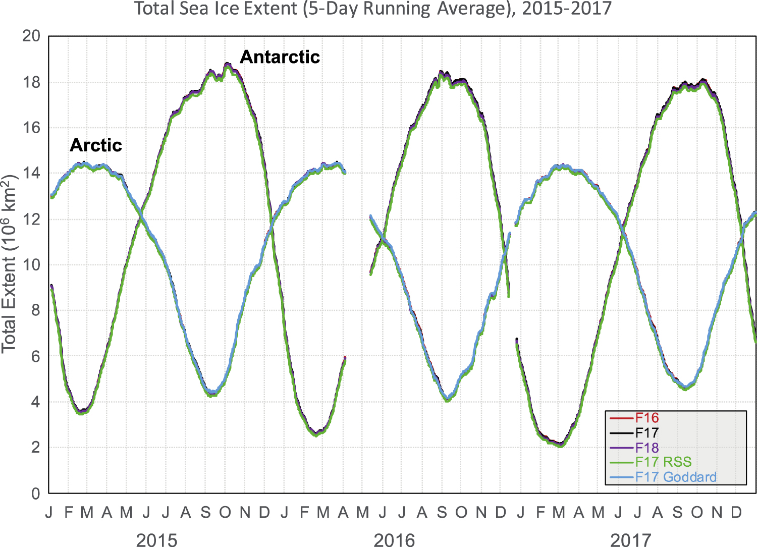
The extent estimates from the product all clearly track the seasonal variability of the ice cover, from a maximum in winter through the summer minimum (figure 1). However, there are clear differences in the estimates from the products and these differences vary seasonally (figure 2). These relate to two primary aspects of the products. First is the sensitivity of the algorithms to emission by different ice conditions, most notably thin ice and surface melt. Surface melt generally reduces concentration (the algorithm interprets the liquid water as open water) and thin ice is underestimated because of emission from the water beneath the ice (Steffen et al 1992). Second, as noted above, the spatial resolution is a key factor in the estimate of extent. Higher resolution products, such as those from AMSR2 will more precisely detect the edge, other factors being equal.
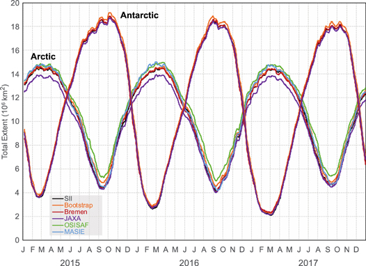
Figure 1. Arctic and Antarctic sea ice extent, 2015–2017, from different products.
Download figure:
Standard image High-resolution image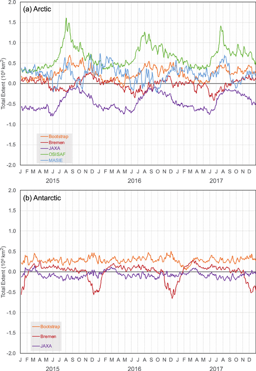
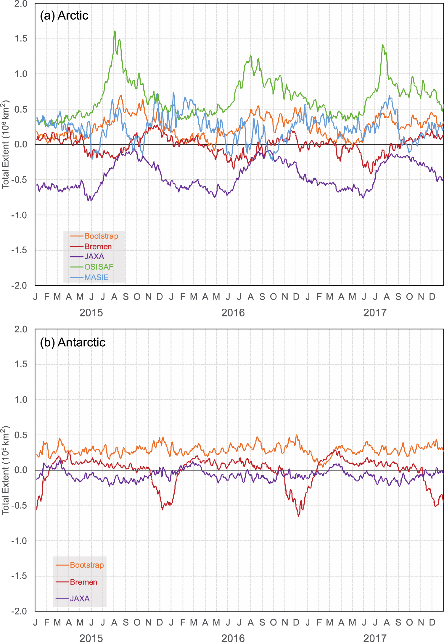
Figure 2. Extent differences between algorithm products and the SII product for (a) Arctic and (b) Antarctic, 2015–2017.
Download figure:
Standard image High-resolution imageOne outlier in the extents is the Ocean and Sea Ice Satellite Application Facility (OSISAF) values in the Arctic, which are as much as 1.5 × 10⁶ km2 above the SII estimates during summer, while other estimates vary within ∼500 000 km2. The reason for this is that the OSISAF version 1 concentration fields do not employ GR weather filters, but instead use atmospheric corrections based on numerical weather model output (Tonboe et al 2016). These corrections remove some weather effects, but some remain, evident as low-concentration (slightly >15%) ice in water regions off the ice edge. These concentrations contribute to the extent, biasing the OSISAF values higher than other products. We note that a soon-to-be-released version 2 of the OSISAF product (Lavergne et al 2019) will include a concentration field with GR filters applied.
Of particular interest are the annual maximum and minimum extent values, especially the Arctic minimum. The focus on the Arctic minimum is due to the significant long-term downward trend observed over the record (since 1979) and the record low minimum extents in 2007 and 2012. It also defines the extent of the multi-year (perennial) sea ice cover. Reduced summer sea ice cover is also of great interest to stakeholders in the region. The minimum and maximum extent show fairly consistent behavior between the products (tables 3 and 4). The Japan Aerospace Exploration Agency (JAXA) is consistently lowest, while OSISAF is highest or second highest (due in part to the weather effects). The SII values are generally close to the middle range of the products. The spread of the extents is nearly one million square kilometers. Roughly half of the spread in the minimum is due solely to the OSISAF product. In winter, both OSISAF and MASIE are higher than the others. The low JAXA values are likely due to the higher spatial resolution, resulting in less 'smearing' of the ice edge; however, this doesn't necessarily mean that JAXA is more accurate—it may miss thin or melting ice and underestimate the ice edge location.
Table 3. Daily (5-day trailing average) minimum and maximum Arctic sea ice extent from different products, 2015–2017. Units are 106 km2. The highest values are highlighted in bold and the lowest values are highlighted in bold-italic.
| Minimum | Maximum | |||||
|---|---|---|---|---|---|---|
| Product | 2015 | 2016 | 2017 | 2015 | 2016 | 2017 |
| SII | 4.43 | 4.17 | 4.67 | 14.52 | 14.51 | 14.41 |
| Goddard | 4.85 | 4.54 | 4.91 | 14.64 | 14.66 | 14.46 |
| Bremen | 4.39 | 4.06 | 4.72 | 14.64 | 14.50 | 14.46 |
| JAXA | 4.31 | 4.03 | 4.49 | 13.92 | 13.92 | 13.85 |
| OSISAF | 5.29 | 5.01 | 5.41 | 14.85 | 14.98 | 14.80 |
| MASIE | 4.53 | 4.30 | 4.66 | 14.85 | 15.04 | 14.75 |
| Median | 4.48 | 4.24 | 4.70 | 14.64 | 14.59 | 14.46 |
| Range | 0.98 | 0.98 | 0.92 | 0.93 | 1.12 | 0.95 |
Table 4. Daily (5-day trailing average) minimum and maximum Antarctic sea ice extent from different products, 2015–2017. Units are 106 km2. The highest values are highlighted in bold and the lowest values are highlighted in bold-italic.
| Minimum | Maximum | |||||
|---|---|---|---|---|---|---|
| Product | 2015 | 2016 | 2017 | 2015 | 2016 | 2017 |
| SII | 3.59 | 2.63 | 2.11 | 18.86 | 18.53 | 18.10 |
| Goddard | 3.86 | 2.88 | 2.27 | 19.18 | 18.87 | 18.43 |
| Bremen | 3.69 | 2.75 | 2.34 | 18.88 | 18.60 | 18.20 |
| JAXA | 3.61 | 2.69 | 2.15 | 18.70 | 18.45 | 17.99 |
| Median | 3.65 | 2.72 | 2.21 | 18.87 | 18.57 | 18.15 |
| Range | 0.27 | 0.25 | 0.23 | 0.48 | 0.42 | 0.44 |
In the Antarctic (table 4), the range in extents is smaller, perhaps due to the fact that OSISAF and MASIE values are not available for the Antarctic. The minimum extent spread is smaller, ∼250 000 km2, than in winter (∼450 000 km2) perhaps simply due to less total ice overall. The larger extent range in winter may be due to the same phenomena—larger extent allows for more variability. There is also a less clear-cut difference between the products with the highest and lowest values varying between maximum and minimum and even the years. The time series of the difference with SII shows interesting features as well (figure 2(b)). The Bootstrap is consistently higher than SII. Bremen and JAXA differences with SII are closer to zero in general, but Bremen has a noticeable drop in the November to February period. This is during austral spring and summer when ice extent is decreasing rapidly. The Bremen product appears to be affected by surface properties (melt) or atmospheric emission (due to the use of the 85–90 GHz channels), which reduce detection of ice relative to the other products.
While the spread of estimates seems large, it reflects a surprisingly small change in ice edge position due to the large perimeter of the ice cover. As demonstrated conceptually in the supplementary materials, a 1 × 10⁶ km2 extent difference reflects a change in ice edge position of only ∼25–75 km (one to three grid cells) depending on the latitude of the ice edge. Also recall that some of the differences, especially those with different gridded resolutions, can be attributed to differences in land masks.
4. Relative uncertainty
While absolute uncertainty is important and is of particular interest to stakeholders operating in the Arctic, in reality the passive microwave data's resolution is too coarse and has too many limitations (thin ice, surface melt) near the ice edge to be very useful to operational users (e.g. Dedrick et al 2001). The primary value of the passive microwave sea ice record is in the long-term tracking of climate trends and variability. For this, the key information is not exactly how much ice there is, but how consistent it is over time. Regardless of the absolute amount of ice, if there is consistency over time then trends and anomalies will be accurate. In other words, it is the relative uncertainty, or precision, that is of most interest for climate monitoring.
Unfortunately, there is no direct way to do this because we have no consistent standard to measure against. Operational ice analyses (such as MASIE, see supplement) would be a possibility, but because they are based on varying data quantity and quality and include subjective assessment by expert ice analysts, they are not a consistent source (Meier et al 2015).
4.1. Approach
The approach here is to investigate the sensitivity of the extent to variations in the processing: (1) NRT versus final processing, (2) different Tb sources, and (3) the GR open water threshold. We use the SII processing scheme as the basis for this assessment. All extents are based on 5-day running averages of daily values, as is done for the published SII values. This smooths out day-to-day variability and yields a more consistent time series. The different inputs are described below and summarized in table 5.
- 1.NRT versus final: NSIDC archives two concentration products. The first is an NRT product (Maslanik and Stroeve 1999) processed at NSIDC that uses NRT Tbs from NOAA CLASS (http://class.noaa.gov/). The second is a final product processed at NASA Goddard (Cavalieri et al 1996) that uses Tbs from Remote Sensing Systems (RSS), Inc. (version 7, Wentz et al 2013; http://remss.com/missions/ssmi/). The different Tb calibration by CLASS and RSS contributes to differences in concentration. In addition, while the concentration algorithm is the same for both the NRT and Goddard product, there are differences in ancillary processing. Goddard fills data gaps with spatial and temporal interpolation and it uses a different ocean mask to filter out false ice retrievals in regions where sea ice never occurs. Finally, it does manual quality control editing to remove clearly spurious ice. The SII extents are derived from the NRT concentrations for recent data, which are replaced with Goddard final data when they become available.
- 2.Tb source: Currently there are three operating SSMIS sensors, on the Defense Meteorological Satellite Program (DMSP) F16, F17, and F18 satellites, all of which have had overlapping operation for the past several years. Though the instruments are the same design, there will be small differences in Tb values due to sensor instrumentation and calibration, as well as observation time. NSIDC has begun processing concentrations from all three sensors internally, though only one sensor (currently F18) is distributed publicly. Also, as noted above, while NSIDC uses CLASS Tbs for its NRT processing, RSS also provides Tbs (albeit not in NRT).
- 3.Weather filter: as noted above, two weather filters are used to automatically remove erroneous ice over open water due to weather effects and these filters potentially affect extent by removing low-concentration ice (potentially including concentrations biased low by melt). The GR2219 was found to only have a small effect on the ice edge (Meier and Ivanoff 2017), so here we investigate only the sensitivity of extent to GR3719. Extent changes due to GR3719 represent sensitivity to both random noise in the Tb values and the ice conditions near the ice edge. The algorithm tiepoints for pure surface type could also be adjusted, which will affect concentration and thus extent, but the weather filter threshold is a more direct and more easily controlled way to test the sensitivity of extent to algorithm parameters.
Table 5. List of the three cases and the parameters that are varied for each. The parameters in bold are common to all three cases and are used as the baseline for comparison.
| Case | Note | Sensor | Tb source | Processed by | GR threshold |
|---|---|---|---|---|---|
| Baseline | NSIDC NRT | F17 | CLASS | NSIDC | 0.05 |
| Goddard | Goddard final | F17 | RSS | Goddard | 0.05 |
| Tb Source | F17 | RSS | NSIDC | 0.05 | |
| F16 | CLASS | NSIDC | 0.05 | ||
| F18 | CLASS | NSIDC | 0.05 | ||
| Weather filter | F17 | CLASS | NSIDC | 0.046 | |
| F17 | CLASS | NSIDC | 0.048 | ||
| F17 | CLASS | NSIDC | 0.052 | ||
| F17 | CLASS | NSIDC | 0.054 |
With the exception of the F17 Goddard final product, all of the test cases above were processed at NSIDC using the same NSIDC processing system that is used for the operational NRT products. We note that the same tiepoints are used for all NSIDC-processed cases, based on the F17 tiepoint values calculated for the NRT CLASS Tb data (Meier et al 2011). Goddard uses different F17 tiepoints, derived based on the RSS Tb data (Cavalieri et al 2012). The Goddard product also made a slight adjustment to the GR3719 weather filter threshold for the Antarctic, from 0.05–0.053.
On 5 April 2016, the F17 SSMIS data started showing spurious behavior due to satellite issues that affected the 37H channel. The channel began operating nominally again on 10 May 2016. This period has been removed from the analysis, as well as a 5-day period in December 2016. One- or two-day periods with missing or bad data occasionally occurred in at least one source; extent values for these days were interpolated from the extents from surrounding days. Details on the missing values are provided in the supplement. The seasonal cycle of all cases is shown for 2015–2017 in figure 3.

Figure 3. Total sea ice extent for the Arctic and Antarctic, 2015–2017, for the Tb source cases. The gaps in the lines represent periods of missing/bad data in April–May and mid-December 2016.
Download figure:
Standard image High-resolution image4.2. Results
The relative uncertainty is estimated by comparing extents from the variant cases with the standard baseline case, which is used as the source for the NRT SII extent estimates. While NSIDC now uses F18 CLASS data for NRT, here we use the F17 CLASS with a 0.05 GR threshold as the baseline. This was selected because (1) it is still (through 2018) used for the Goddard product, (2) it was the near-time-standard for several years until the satellite issues in April 2016, (3) RSS has not yet provided F18 SSMIS data, and (4) NSIDC has not distributed F16 data publicly. So, it is the one configuration that can be compared consistently across all other cases.
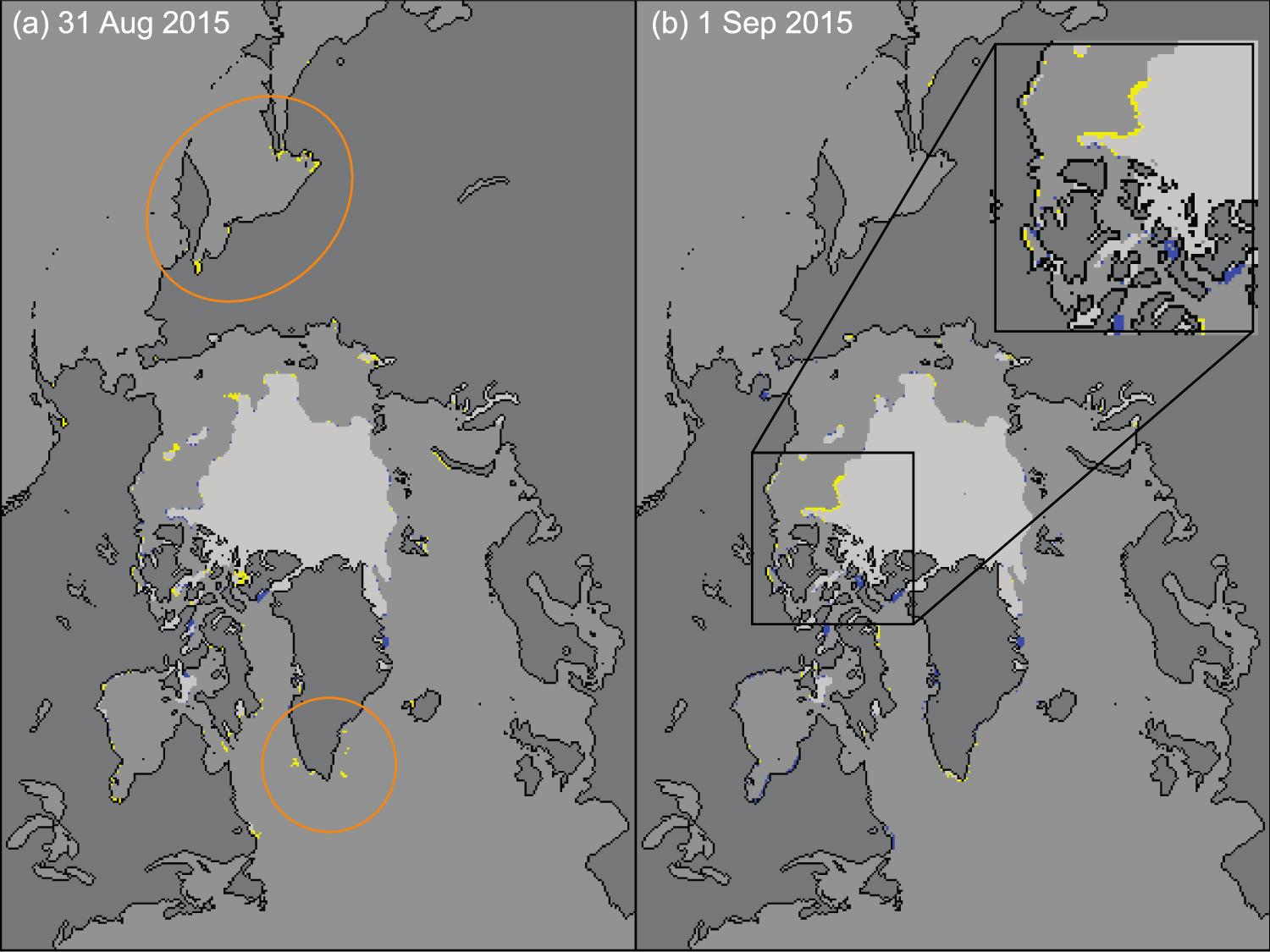
The first uncertainty is simply in how much extent changes when the NRT concentration source is replaced by the final Goddard concentration fields. A notable feature in the Goddard differences (figure 4(a)) are small sudden jumps that occur at month transitions (e.g. April to May 2015 and August to September 2015). This occurs due to the difference in ocean masks used in the Arctic to filter residual weather effects far from the ice edge where sea ice is not possible. Goddard uses a sea surface temperature-based monthly climatology (Cavalieri et al 1996). NSIDC found that this climatology was too conservative and allowed too much false ice in the NRT product, particularly during summer with the much lower than average extents in recent years. Goddard does manual corrections to remove such false ice, so the conservative climatology is not a problem for clearing out weather effects—they are removed manually. However, much of the false ice occurs along the coast due to mixed ocean–land sensor footprints. As noted in the supplement, a filter removes some of this effect, but not all of it. The ocean masks are monthly fields and a change in month marks a transition to a new ocean mask. So, the differences in the ocean masks result in a different amount of coastal ice being removed in a given month, which causes the sudden, small jumps in the Goddard extent difference. This is shown in figure 5, where coastal ice in the Sea of Okhotsk and weather effects off southern Greenland are evident in the NRT extent field on 31 August, but not on 1 September.

Figure 4. Extent difference of Tb source cases with the NSIDC baseline case.
Download figure:
Standard image High-resolution image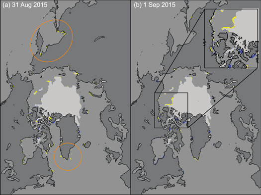
Figure 5. Map of extent comparison between Goddard and NSIDC NRT sources. Yellow indicates grid cells where only NSIDC has ice, blue indicates grid cells where only Goddard has ice. Gray grid cells show no difference between Goddard and NSIDC with shade varying from light gray (100% ice), medium gray (0% ice), dark gray (land), to black (coastline). Circled in orange are regions where NSIDC shows ice on 31 August, but not 1 September due to changes in the ocean mask. The inset in (b) zooms in on a region in the Beaufort Sea and Canadian Archipelago to show more detail on the small differences.
Download figure:
Standard image High-resolution imageWhile the bias between the Goddard and the NRT daily (5-day running average) values is overall fairly small (table 6), it varies by month and during September in the Arctic it is ∼41 000 km2. This is largely due to coastal ice from land spillover, as seen in figure 5. There is also variability (standard deviation) in the daily extent values (table 7), which adds further to the uncertainty. Taken together, the uncertainty in NRT extents relative to the Goddard final values is ∼100 000 km2 using a two standard deviation range for uncertainty. Note that this uncertainty only exists for the time when NRT values are used. Once the NRT values are replaced by final values from Goddard (6–12 months later), this uncertainty disappears.
Table 6. Mean difference (bias) with F17 CLASS (GR = 0.05) baseline extent. Units are 106 km2.
| Period | Goddard | F17 RSS | F16 | F18 | GR0.046 | GR0.048 | GR0.052 | GR0.054 |
|---|---|---|---|---|---|---|---|---|
| Arctic | ||||||||
| All | 0.018 | −0.123 | 0.013 | −0.021 | −0.025 | −0.010 | 0.007 | 0.011 |
| March | 0.001 | −0.122 | −0.013 | −0.007 | −0.023 | −0.010 | 0.007 | 0.012 |
| September | 0.041 | −0.164 | −0.005 | −0.019 | −0.021 | −0.008 | 0.006 | 0.009 |
| Antarctic | ||||||||
| All | 0.007 | −0.175 | −0.007 | −0.051 | −0.030 | −0.011 | 0.006 | 0.010 |
| February | −0.009 | −0.126 | −0.002 | −0.031 | −0.020 | −0.007 | 0.005 | 0.008 |
| September | 0.012 | −0.182 | −0.005 | −0.059 | −0.039 | −0.014 | 0.007 | 0.011 |
Table 7. Difference standard deviation with F17 CLASS (GR = 0.05) baseline extent. Units are 106 km2. Values in bold are used in the estimate of relative uncertainty in section 4.3.
| Period | Goddard | F17 RSS | F16 | F18 | GR0.046 | GR0.048 | GR0.052 | GR0.054 |
|---|---|---|---|---|---|---|---|---|
| Arctic | ||||||||
| All | 0.043 | 0.029 | 0.032 | 0.025 | 0.010 | 0.004 | 0.003 | 0.005 |
| March | 0.015 | 0.011 | 0.022 | 0.015 | 0.006 | 0.003 | 0.004 | 0.007 |
| September | 0.024 | 0.027 | 0.017 | 0.011 | 0.006 | 0.003 | 0.002 | 0.004 |
| Antarctic | ||||||||
| All | 0.024 | 0.054 | 0.019 | 0.030 | 0.019 | 0.007 | 0.004 | 0.007 |
| February | 0.012 | 0.010 | 0.018 | 0.023 | 0.005 | 0.002 | 0.002 | 0.004 |
| September | 0.014 | 0.033 | 0.030 | 0.020 | 0.010 | 0.004 | 0.002 | 0.004 |
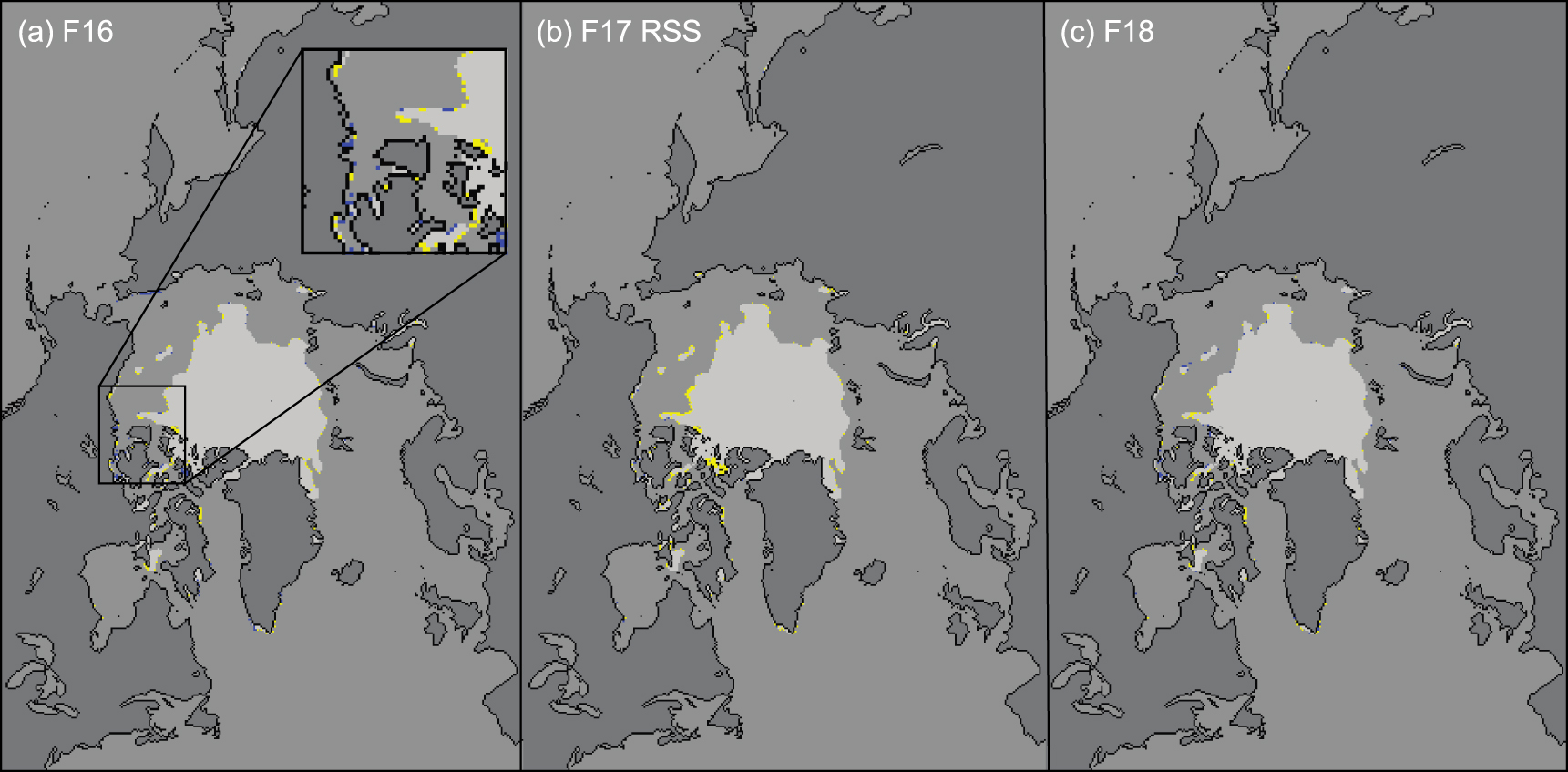
In looking at the sensitivity to Tb, the first noticeable feature is a clear bias in the extents using RSS Tbs (figure 4). This is not surprising because, as noted above, the NSIDC processing uses the same tiepoints, derived for the F17 CLASS data. These tiepoints are not optimal for the RSS data, which results in the bias. Biases are much smaller for the extents from the F16 and F18 SSMIS Tbs. Spatially, the differences in extent are small, mostly scattered points along the coast and the ice edge (figure 6). The F17 RSS case (figure 6(b)) shows the most noticeable difference in the Beaufort Sea near Banks Island, where the ice edge is retracted poleward by a few grid cells. This is due to the inappropriate tiepoints for the RSS Tb input.
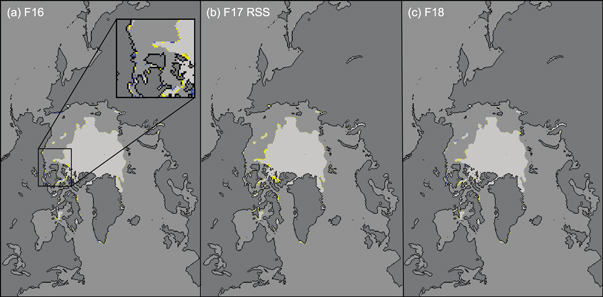
Figure 6. Comparison maps of extent for (a) F16, (b) F17 RSS, and (c) F18. Yellow indicates cells where ice occurs only in the baseline cases. Blue indicates cells where ice occurs only in the comparison case.
Download figure:
Standard image High-resolution imageThe extent differences for the GR threshold changes are much smaller in magnitude than the Tb source comparison (figure 7). The bias clearly changes with GR threshold because the threshold allows more or less ice (i.e. it shifts the effective minimum concentration threshold). There is greater sensitivity at lower GR values than at the higher GR values. This makes sense because the lower GR values correspond to a more stringent filter that effectively raises the minimum concentration that is allowed. As it raises that minimum concentration above 15%, the total extent will be directly affected. Raising the GR threshold will filter less weather and will lower the minimum detectable concentration, but there are usually relatively few weather effects and if the threshold corresponds to a concentration <15%, it will not affect the total extent. This is seen in spatial maps of extent where the lower threshold values very clearly cut off ice compared to the baseline case, but higher thresholds have little noticeable effect on the ice edge (figure 8). Antarctic extents are more sensitive to GR, particularly during the major ice growth period of September–December. The higher sensitivity is partly due to the large perimeter of ice as it expands to encircle the entire continent; it also likely reflects a sensitivity to thin ice growth at the edge as well as potentially strong atmospheric effects over the Southern Ocean.

Figure 7. Extent difference with the baseline case for different GR threshold values for (a) Arctic and (b) Antarctic.
Download figure:
Standard image High-resolution image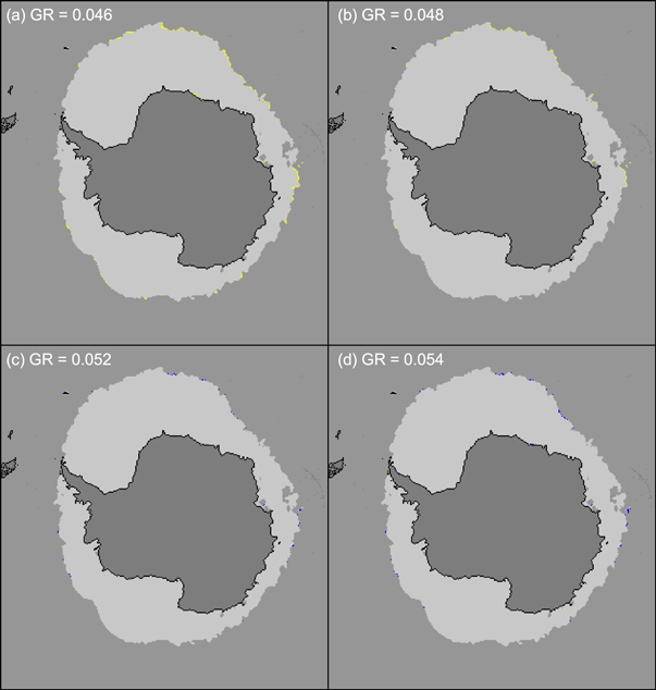
Figure 8. Comparison maps of extent for GR thresholds of (a) 0.046, (b) 0.048, (c) 0.052, and (d) 0.054. Yellow indicates cells where ice occurs only in the baseline cases. Blue indicates cells where ice occurs only in the comparison case.
Download figure:
Standard image High-resolution image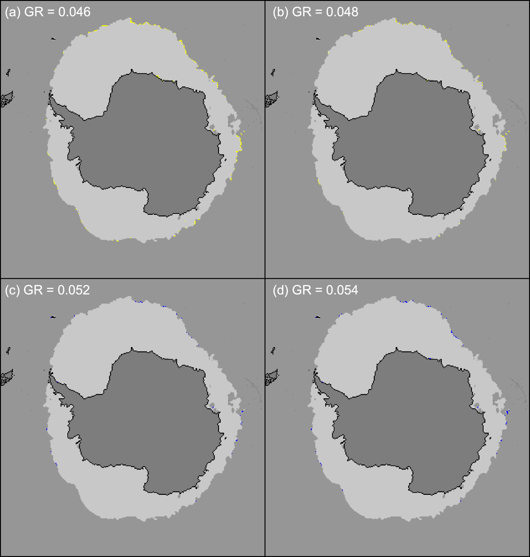
We note that the chosen range of GR threshold adjustment (±0.02, ±0.04) is somewhat arbitrary. Adjusting it more would obviously increase the magnitude of the extent differences. The rationale for our selection is that the open water points generally cluster within a 0.02 range of GR values (Steffen et al 1992) and when the GR threshold has been adjusted to optimize consistency between sensors, the adjustments have been within ±0.04 (Cavalieri et al 2012, Meier and Ivanoff 2017).
4.3. Estimating relative uncertainty
In the previous section, we estimated the sensitivity of the extent to changes in parameters for three different configurations. While the NRT versus Goddard difference is largest (both bias and standard deviation), this uncertainty only applies when comparing NRT extent values with Goddard values from previous years. Thus, we consider this a separate uncertainty from the 'internal' uncertainty that affects any extent estimate.
The Tb source uncertainty is indicated by the variation (standard deviation) due to different sources: F17 RSS, F16 CLASS, and F18 CLASS. The differences are due to the different Tb calibration (RSS versus CLASS) or different orbit/sensor properties (different observation times and CLASS calibrations for F16, F17, and F18).
In general, biases between sensors, even remaining biases after intercalibration, do increase uncertainty when comparing extents between different sensors. But for uncertainty of extents from a given product/source (same sensor, same algorithm), the biases between sensors or processing are not relevant, so we use only the standard deviation as the basis for uncertainty. In other words, using the standard deviation of differences from varying sources and algorithm parameters simulates the uncertainty from a single source and set of algorithm parameters.
In terms of estimating total uncertainty, the most straightforward approach is to assume the uncertainties from the Tb sources and the weather filters are independent. In practice, the GR threshold will be affected by the Tb source, but for simplicity we ignore this. To calculate a total uncertainty, we first average the Tb uncertainties (since all configurations are simply different ways of estimating the sensitivity to Tb). Next, we average the GR threshold uncertainty from the ±0.04 GR range. Then we estimate the total uncertainty via a sum of squares of the Tb source and GR average standard deviations (equation (1)):
The total uncertainty is calculated as an overall average for the entire three-year time period and for the months of September and February (Antarctic) or March (Arctic). These pairs of months are of particular interest because it is when the minimum and maximum extents normally occur (table 8).
Table 8. Average of standard deviations for the Tb source cases (F17 RSS, F16, F18), the GR cases (±0.04), and the total based on equation (1). Values in bold text represent the final relative uncertainty estimates. Units are 106 km2. Values are rounded to the nearest 0.001 (1000 km2).
| Period | Tb source | GR | Total st. dev. | Uncertainty range |
|---|---|---|---|---|
| Arctic | ||||
| All | 0.029 | 0.008 | 0.030 | 0.060 |
| March | 0.016 | 0.007 | 0.017 | 0.034 |
| September | 0.018 | 0.005 | 0.019 | 0.038 |
| Antarctic | ||||
| All | 0.034 | 0.013 | 0.036 | 0.072 |
| February | 0.017 | 0.005 | 0.018 | 0.036 |
| September | 0.027 | 0.006 | 0.028 | 0.056 |
A common standard for an uncertainty is the 2σ range, the rightmost column in table 8. As noted above, this an uncertainty for a constant sensor and constant processing method. For the NSIDC SII, these uncertainties would be most valid for comparing extents with the same processing method (Goddard or NSIDC NRT) and the same sensor (F17). Currently, the SII values from 2008–2017 are based on Goddard values processed using F17.
Of particular interest to scientists and the general public is the September minimum extent in the Arctic. One application of these uncertainties is to assess these September minimums in light of the calculated uncertainties. Table 9 shows the ten lowest minimum extents (through 2017) with the rankings considering the uncertainty range. Our assessment is that years that have extents within 2σ of each other should be considered to be tied.
Table 9. Ranking of Arctic minimum sea ice extents from the NSIDC SII. 'T' indicates a tie, i.e. the values are within the 2σ uncertainty range of each other.
| Rank | Year | Extent |
|---|---|---|
| 1 | 2012 | 3.39 |
| 2 T | 2007* | 4.16 |
| 2 T | 2016 | 4.17 |
| 4 | 2011 | 4.34 |
| 5 | 2015 | 4.43 |
| 6 T | 2008 | 4.59 |
| 6 T | 2010 | 4.61 |
| 8 | 2017 | 4.67 |
| 9 T | 2014 | 5.03 |
| 9 T | 2013 | 5.05 |
*Note that the 2007 extent is from the F13 SSMI sensor, while others are from F17 SSMIS. This increases the uncertainty due to intercalibration. Units are 106 km2.
As discussed above, these uncertainties assume a consistent sensor and processing. So, they are most valid for comparing extents from a single source. Transitions between different sensors introduce further uncertainty, which depends on the quality of the intercalibration. Meier et al (2011) found that these inconsistencies were in part due to limited overlap periods. In a later study, Eisenman et al (2014) noted inconsistencies in the time series attributable to intercalibration, particularly in the early part of the record. Unlike early transitions, the F13 SSMI to F17 SSMIS intercalibration had a full year of overlap to derive adjustments. This led to a high-quality intercalibration and only very small errors (Meier et al 2011, Cavalieri et al 2012). Another concern is 'sensor drift'. Over time, the orbits of satellites will change due to atmospheric drag. This will change observation times and altitude. These could change the performance within a sensor over time. Fortunately, F13 and F17 had only minimal orbital drift, so this error should be small. Thus, there should be good confidence in the above-derived uncertainty estimates since the beginning of the F13 SSMI in 1995.
5. Discussion and conclusion
Since at least 2007, interest in Arctic sea ice extent, particularly the maximum and minimum seasonal extremes, has been growing. The record low extents in 2007 and 2012 brought considerable attention to the long-term sea ice decline. More recently, record low and record high extents in the Antarctic have turned attention to the southern hemisphere sea ice as well. The changing ice is impacting stakeholders, from native communities to commercial interest. In response, two efforts have evolved. The NSIDC Arctic Sea Ice News and Analysis (https://nsidc.org/arcticseaicenews/), funded by NASA, provides daily updates of extent based on the NSIDC SII and regular real-time analyses of conditions through the year. The Sea Ice Outlook (https://arcus.org/sipn/sea-ice-outlook), coordinated by the Arctic Research Consortium of the United States and funded by multi-agency international partners, solicits contributions from the community to make predictions of the Arctic September (and more recently Antarctic February) extent. The prediction methods vary from geophysical models, statistical methods, and heuristic approaches. Many are initialized by passive microwave sea ice extent/concentration fields. The predictions are evaluated relative to the NSIDC SII extents.
While the SII values are widely used in the science community, they do not represent better or more accurate estimates compared to other products. The goal of this paper is to put the SII extents in a more general context. We have provided an estimate of an absolute uncertainty range of extents, based on the output from several different products. These suggest a range of 500 000 to 1 × 10⁶ km2 in extent from the different products. This range can be explained by biases in ice edge position of 25–75 km due to differences in sensitivity of the algorithms to conditions near the ice edge (e.g. thin ice) and sensor spatial resolution.
Relative uncertainty was assessed through an analysis of variations in the SII processing, adjusting the input Tb source and algorithm parameters (GR weather filter threshold). The relative uncertainties are 30 000–70 000 km2 depending on the time of year and hemisphere for a given sensor. For the Arctic September minimum extent, the uncertainty was found to be 38 000 km2. Slightly higher ranges are expected for comparisons between different sensor sources, though the stability of the time series appears to be good since the start of the F13 record in 1995. There is a larger uncertainty between NRT and final processing by Goddard. Thus, NRT extent estimates should be considered with more caution when comparing to earlier estimates based on Goddard concentration fields.
Ideally, a fully independent, high-quality, consistent, hemisphere-wide validation product would be used as a true estimate of extent to compare the passive microwave derived extents. However, such a product does not exist. Operational ice charts are high quality, but because their input data quality and quantity vary and because they use manual analysis the fields are not consistent over time. The approach used here to estimate uncertainty is intrinsic to the data sources themselves and may not encompass the full range of uncertainty.
This analysis is focused on hemisphere-wide extent uncertainty. Regional conditions are often important to specific stakeholders. Regional extent uncertainties may be larger because there could be offsetting (high and low) biases in different regions that tend to cancel each other in the hemisphere-wide values. We plan to investigate regional uncertainties in a follow-on study.
The passive microwave sea ice record is one of the longest satellite-derived climate records and one of the most iconic indicators of climate change. However, this long-term record is threatened. The existing passive microwave sensors used by the community for sea ice extent are aging. As of this paper (December 2018), the newest sensor, AMSR2, is over six years old, already past its nominal 5-year mission. The current DMSP SSMIS sensors have been operating at least eight years, and the oldest (on F16) was launched more than 14 years ago. The US Department of Defense, JAXA, and the European Space Agency have plans to launch new passive microwave sensors, but these are in their incipient stages and the earliest launch is likely to be at least five years in the future. China has a passive microwave sensor on its FY-3C satellite and future launches are planned. However, there is still a growing potential for a gap in the passive microwave record. If such a gap occurs, intercalibration between sensors would not be possible and the quality of the long-term sea ice extent climate indicator would be degraded. This would be a significant loss to the climate monitoring community.
Acknowledgments
This work was supported by the Sea Ice Prediction Network (SIPN) project, funded by the NSF (Grant #PLR1304246) and through the NASA Distributed Active Archive Center at the National Snow and Ice Data Center (Contract #80GSFC18C0102). Thanks to T Lavergne, Norwegian Meteorological Institute, for OSISAF extents and R Gersten, NASA Goddard Space Flight Center, for Bootstrap extents.
Government rights notice
This work was authored by employees of the National Snow and Ice Data Center at the University of Colorado, Boulder under Contract No. 80GSFC18C0102 with the National Aeronautics and Space Administration. The United States Government retains and the publisher, by accepting the article for publication, acknowledges that the United States Government retains a non-exclusive, paid-up, irrevocable, worldwide license to reproduce, prepare derivative works, distribute copies to the public, and perform publicly and display publicly, or allow others to do so, for United States Government purposes. All other rights are reserved by the copyright owner.