

Abstract
Warm periods in Earth's history tend to cool more slowly than cool periods warm. Here we explore initial differences in how the global ocean takes up and gives up heat and carbon in forced rapid warming and cooling climate scenarios. We force an intermediate-complexity earth system model using two atmospheric CO2 scenarios. A ramp-up (1% per year increase in atmospheric CO2 for 150 years) starts from an average global CO2 concentration of 285 ppm to represent warming of an icehouse climate. A ramp-down (1% per year decrease in atmospheric CO2 for 150 years) starts from an average global CO2 concentration of 1257 ppm to represent cooling of a greenhouse climate. Atmospheric CO2 is then held constant in each simulation and the model is integrated an additional 350 years. The ramp-down simulation shows a weaker response of surface air temperature to changes in radiative forcing relative to the ramp-up scenario. This weaker response is due to a relatively large and fast release of heat from the ocean to the atmosphere. This asymmetry in heat exchange in cooling and warming scenarios exists mainly because of differences in the response of the ocean circulation to forcing. In the ramp-up, increasing stratification and weakening of meridional overturning circulation slows ocean heat and carbon uptake. In the ramp-down, cooling accelerates meridional overturning and deepens vertical mixing, accelerating the release of heat and carbon stored at depth. Though idealized, our experiments offer insight into differences in ocean dynamics in icehouse and greenhouse climate transitions.
Export citation and abstract BibTeX RIS

Original content from this work may be used under the terms of the Creative Commons Attribution 3.0 licence. Any further distribution of this work must maintain attribution to the author(s) and the title of the work, journal citation and DOI.
1. Introduction
The characteristics of ocean water masses regulate the exchange of heat and carbon between the ocean and the atmosphere. These characteristics include water mass initial heat and carbon inventories (Winton et al 2013, Ödalen et al 2018) and capacity for additional storage (Xie and Vallis 2012, Ödalen et al 2018), which is set by circulation (Banks and Gregory 2006, Xie and Vallis 2012, Winton et al 2010, 2013, Ödalen et al 2018) and the relative strength of physical and biological ocean carbon pumps (Ödalen et al 2018). Ocean/atmosphere heat and carbon exchange is not necessarily coupled spatially (e.g. Frölicher et al 2015) or temporally (e.g. Garuba et al 2018). The Southern Ocean is presently a primary region of anthropogenic heat and carbon uptake, whereas anthropogenic carbon storage is spread across lower latitudes, and anthropogenic heat storage is more restricted to the upper ocean, and is greatest in the Southern and Atlantic Oceans (Frölicher et al 2015). Similar spatial patterns have been found in natural variability of carbon and heat storage by Thomas et al (2018), who described the variability as a function of convective states in the Weddell Sea. Regional changes in ocean circulation brought about by climate warming might affect the regional ocean heat uptake, resulting in changes to the global atmospheric temperature warming rate (Garuba et al 2018).
Ocean heat and carbon uptake has relevance to metrics commonly used to assess climate responses to external forcing. These concepts generally seek to characterize the response of global mean temperature to a change in atmospheric CO2 (Intergovernmental Panel on Climate Change 2014). Two examples of metrics are: equilibrium climate sensitivity, or ECS, which scales equilibrium surface temperature response against a forced change in atmospheric CO2 concentration, and transient climate response, or TCR, which scales transient warming against a forced change in atmospheric CO2 concentration. Such metrics can be used to inform projections of future climate change (e.g. Meinshausen et al 2008). However, recent work has demonstrated they exhibit initial state-dependent qualities, particularly over longer timescales. For example, data suggest ECS (defined here as the global equilibrium surface temperature response for a change in radiative forcing) may have been 30%–40% lower than intermediate glacial states during fully glacial states, and there is limited evidence of reduced sensitivity to land ice albedo feedback in other colder-than-modern climates (summarized by von der Heydt et al 2016). TCR has similarly been shown to be sensitive to initial climate state (e.g. Weaver et al 2007, He et al 2017), in which ocean circulation state (He et al 2017) (and specifically, the strength and depth of the Atlantic Meridional Overturning Circulation; Kostov et al 2014), exerts control on the modelled ocean heat uptake efficacy (Winton et al 2010, He et al 2017).
Understandably, the majority of the attention paid to climate metrics and the decoupling of ocean/atmosphere heat and carbon uptake is in warming modern and glacial climates. While modern or close-to-modern warming studies have obvious relevance, studies of other climate states also have value for understanding heat and carbon dynamics. Here we extend the general discussion of ocean/atmosphere exchange to a comparison of the heat and marine carbon dynamical responses to rapidly warming an equilibrated icehouse (pre-industrial atmospheric CO2 concentration, strong deep ocean circulation, low ocean suboxia) and rapidly cooling an equilibrated greenhouse (higher-than-modern atmospheric CO2 concentration, weaker deep ocean circulation, higher ocean suboxia) climate, in order to improve our understanding of the ocean dynamics regulating heat and carbon storage and exchange. A greenhouse climate is interesting because presently our icehouse earth is warming, and is likely committed to future reductions of Atlantic Meridional Overturning Circulation, polar ice, and oceanic oxygen (Intergovernmental Panel on Climate Change 2014). These changes indicate a transition toward a greenhouse climate state, which is possibly the most stable (and therefore, the most difficult to transition out of) of the climate states (Kidder and Worsley 2010). We force our model using values for atmospheric CO2 concentration within a range consistent with the climate literature (modern icehouse, 285 ppm; Intergovernmental Panel on Climate Change 2014, and hypothetical greenhouse within the likely range of the Early Eocene Climate Optimum, 1257 ppm; Anagnostou et al 2016). We employ symmetric increases and decreases in prescribed atmospheric CO2 concentrations for a direct comparison of two hypothetical transitions between climate states, in order to investigate the relative symmetry of the transitions.
2. Model description and experiments
For our experiments we use the University of Victoria Earth System Climate Model (UVic ESCM) version 2.9 (Weaver et al 2001, Meissner et al 2003, Eby et al 2009, Schmittner et al 2005b, 2008). It contains an ocean model, land and vegetation components, dynamic-thermodynamic sea ice model, and sediments. The atmosphere is represented by a two-dimensional energy-moisture balance model. Winds are prescribed from monthly NCAR/NCEP reanalysis data and are adjusted geostrophically to surface pressure changes (Weaver et al 2001). Continental ice sheets are fixed. The UVic ESCM has a horizontal resolution of 3.6° longitude × 1.8° latitude, with 19 vertical levels in the ocean. We use an updated NPZD-type marine biogeochemical model (Keller et al 2012).
We first integrate the model 20 000 years in two configurations to achieve equilibrium climate states. The first configuration, for the ramp-up experiment (hereafter, WARMING), is equilibrated with an atmospheric CO2 concentration of 285 ppm to represent an icehouse climate. The second, for the ramp-down experiment (hereafter, COOLING), is equilibrated with an atmospheric CO2 concentration of 1257 ppm to represent a greenhouse climate. Solar and orbital forcing is prescribed at modern levels in each configuration.
We then force each respective configuration with a 1% per year increase (for WARMING) or 1% per year decrease (for COOLING) in atmospheric CO2 concentration for 150 years to reach the other experiment's initial CO2 concentration (figure 1). Each model is then integrated an additional 350 years, keeping atmospheric CO2 concentrations fixed at year 150 levels. No changes in non-CO2 greenhouse gas forcings are included in the simulations.

Figure 1. Atmospheric CO2 forcing used for WARMING (dark blue) and COOLING (light blue) experiments.
Download figure:
Standard image High-resolution image3. Comparison and discussion of WARMING and COOLING results
Experiment WARMING has an initial average surface air temperature (SAT) of 14.2 °C and an average ocean temperature of 4.1 °C. Experiment COOLING is much warmer, and has an initial average SAT of 21.5 °C and an average ocean temperature of 10.2 °C. Initial COOLING sea ice is restricted to patches in the Arctic Ocean and the Ross and Weddell Seas (not shown). Initial ocean convection in COOLING compared to WARMING is stronger in the Ross and Weddell Seas (with annual mean ventilation depths—defined as the depth of potential instability—exceeding 400 m versus 100 m), and in the North Atlantic region it is more restricted to the Nordic Seas (not shown). The initial greenhouse ocean in COOLING is better ventilated than the initial icehouse ocean in WARMING, as evidenced by a higher average radiocarbon value (−77.2 versus −129.9 per mil). A more globally ventilated greenhouse ocean is produced by the stronger wind forcing in this configuration.
3.1. Global climate responses to CO2 forcing
Figure 2 shows the global mean responses in WARMING and COOLING to the CO2 forcings. SAT increases with increasing atmospheric CO2 concentrations in WARMING, and continues to increase after CO2 is held constant, because of inertia in the climate system (Eby et al 2009). Likewise, SAT decreases with decreasing atmospheric CO2 concentrations in COOLING. Gaps between end points in WARMING and COOLING indicate neither simulated SAT has yet reached equilibrium with the final CO2 concentration. Warming during WARMING is about 1 °C greater than cooling during COOLING within the 500 years of integration, and is reflected in the higher WARMING proportion of surface warming to radiative forcing (shown here as ΔSAT/ΔR, where R stands for radiative forcing). Previous work has demonstrated a nonlinear transient climate response to cumulative emissions relationship in the negative phase of CO2 removal scenarios (Zickfeld et al 2016). This nonlinearity occurs because of the inertia of the ocean, so the ocean continues to take up heat and carbon after atmospheric CO2 concentrations have started to decline (Zickfeld et al 2016). In our simulations, the cumulative diagnosed emissions for WARMING is 4305 Pg C over the 500 year integration, and −5472 Pg C over the 500 year integration in COOLING. Our simulations start from equilibrium and are therefore affected by a different mechanism (noted but not described by Zickfeld et al (2016)), which we describe in detail in the following.

Figure 2. Global responses in the WARMING (dark blue) and COOLING (light blue) experiments: global average SAT plotted against atmospheric CO2 concentrations (top left), global average proportion of surface warming to radiative forcing ΔSAT/ΔR (top middle), maximum overturning in the Atlantic (top right), global average ocean heat uptake plotted against atmospheric CO2 concentrations (bottom left), global average ocean carbon uptake plotted against atmospheric CO2 concentrations (bottom middle), and maximum AABW overturning (bottom right). Negative flux values indicate flux out of the ocean and into the atmosphere and negative overturning values indicate anti-clockwise rotation. Increasing time is indicated by arrows on the CO2-dependent plots.
Download figure:
Standard image High-resolution imageDifferences in the proportion of surface warming to radiative forcing in WARMING and COOLING are produced by asymmetric ocean heat responses, brought about by differing ocean dynamics described in the next section. During COOLING, the magnitude of the oceanic release of heat and carbon (shown as negative fluxes in figure 2) is larger than the magnitude of uptake by the WARMING ocean. In COOLING, the rate of release also accelerates throughout the period of transient CO2, whereas during WARMING the oceanic uptake of heat and carbon decelerates. The release of ocean heat to the atmosphere in COOLING has a warming effect on SAT, while atmospheric CO2 concentrations are forced to decline in our simulations, regardless of oceanic carbon outgassing. Similarly, the uptake of heat by the ocean in WARMING has a cooling effect on SAT. In both scenarios the exchange of heat works to damp the response. However, this is not the case for carbon exchange, which is decoupled because of prescribed atmospheric CO2 concentrations and therefore has no impact on the radiative forcing. The large-scale ocean dynamics are described below.
3.2. Response of ocean circulation to CO2 forcing
Decelerating global heat and carbon fluxes in WARMING can be partly explained by a reduction in northern hemisphere overturning over the course of the integration (upper right panel of figure 2), which reduces air-sea gas and heat exchange. Increasing stratification and a reduction of overturning circulation with increasing atmospheric CO2 concentrations is a common result in model studies using modern boundary conditions, e.g. Sarmiento et al (1998), Bopp et al (2005), Schmittner et al (2005a), Weaver et al (2007), Schmittner et al (2008), Steinacher et al (2010). Accelerating global heat and carbon fluxes in COOLING can likewise be partly explained by a strengthening of overturning in both northern and southern hemispheres (right panels of figure 2).
Basin-averaged plots of meridional overturning in figure 3 show the effect of weakening/strengthening convection in WARMING and COOLING. In WARMING, North Atlantic Deep Water (NADW) formation weakens and shoals and Antarctic Bottom Water (AABW) formation nearly collapses, similar to other previously published increasing atmospheric CO2 concentration experiments using the UVic ESCM (e.g. Weaver et al 2007, Schmittner et al 2008). In COOLING, initial overturning plots display a maximum North Atlantic meridional overturning strength of 18 Sv that extends to 3000 m depth (globally averaged), and a maximum AABW overturning strength of 12 Sv. As atmospheric CO2 levels decrease, the NADW cell strengthens from 18 to 38 Sv and extends downwards to reach the vertical extent of the North Atlantic. AABW in the Indo–Pacific also strengthens, reaching 26 Sv at the end of the transient CO2 forcing, and extends northward to most of the basin. In both hemispheres, strengthening of the overturning during COOLING is achieved by a surface cooling and salinification in the polar deep water formation regions over the course of the integration (not shown). The strongly asymmetric response of the ocean circulation in WARMING and COOLING is due to the different initial states and the different CO2 forcing. In WARMING, the cool ocean warms from the surface, which increases stratification and reduces overturning. In COOLING, the relatively warmer ocean is cooled from the surface, which temporarily accelerates overturning.

Figure 3. Initial and year 150 meridional overturning circulation for WARMING (left columns) and COOLING (right columns). Contours denote intervals of 2 Sv. Negative values are shown as dotted lines and represent anti-clockwise rotation.
Download figure:
Standard image High-resolution image3.3. Response of ocean heat and carbon storage to changes in circulation
Thermal and carbon anomalies in WARMING and COOLING oceans (figures 4 and 5, where DIC stands for dissolved inorganic carbon) are primarily a product of both the changing atmospheric CO2 concentrations as well as the response of the ocean circulation. This is suggested by the fact that at a basin scale, the DIC responses well match the concurrent responses in radiocarbon (of which the atmospheric concentration is held at 0, figure 6). In WARMING, the rising heat content is limited to the upper half of the global ocean. This has a damping effect on air-sea fluxes, reducing uptake rates. Carbon anomalies are strongest in the upper half of the Atlantic. This is because AABW continues to form, albeit more slowly, therefore overall raising the DIC content. The Pacific develops a thermal anomaly profile similar to the Atlantic due to the surface North Pacific taking up the rising atmospheric heat while the deep water circulation slows. The strongest DIC anomalies occur in the subtropical gyres. Strong sub-surface warming occurs in the Indian Ocean as heat is advected by the currents moving west out of the central-western Pacific. Surface temperature anomalies are strongest in the high latitudes (due to ice-albedo feedback) and western basins (regions dominated by fast poleward surface currents), while surface carbon anomalies are strongest in the central basin gyres. Strongest accumulation of carbon in the gyres agrees with the fifth phase of the Coupled Model Intercomparison Project (CMIP5) multi-model comparison of anthropogenic carbon uptake of Frölicher et al (2015). The gyre regions do not take up the carbon directly; rather the carbon is advected laterally from the high latitudes (Frölicher et al 2015). Strong Southern Ocean temperature anomalies also agree with the intermodel comparison of Frölicher et al (2015) demonstrating the Southern Ocean as an important anthropogenic heat uptake and storage location.
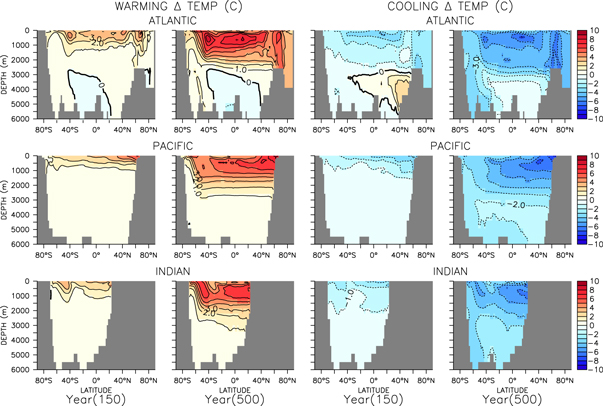
Figure 4. Changes in WARMING (left columns) and COOLING (right columns) zonal average ocean temperature for the Atlantic, Pacific and Indian basins after 150 and 500 years of simulation.
Download figure:
Standard image High-resolution image
Figure 5. Changes in WARMING (left columns) and COOLING (right columns) zonal average ocean DIC for the Atlantic, Pacific and Indian basins after 150 and 500 years of simulation.
Download figure:
Standard image High-resolution image
Figure 6. Changes in WARMING (left columns) and COOLING (right columns) zonal average ocean background radiocarbon for the Atlantic, Pacific and Indian basins after 150 and 500 years of simulation.
Download figure:
Standard image High-resolution image
In COOLING, thermal anomalies roughly mirror those found in WARMING, but carbon anomalies differ substantially. Deepening of Atlantic meridional overturning reduces the separation of intermediate and deep water masses, warming and ventilating the deep ocean. This effect is transient, and by year 500 the positive thermal anomaly is no longer apparent in the zonal average. The strongest cooling occurs in the upper half of the Atlantic, due to decreasing SAT and oceanic heat release, as well as the upward mixing of cooler deep water. However, the stronger ventilation of deep water produces a carbon anomaly that is strongest below 3000 meters. Over the period of equilibration at 1257 ppm atmospheric CO2, a large amount of carbon accumulated in the deep ocean. When Atlantic meridional overturning accelerates, this carbon is quickly brought up into the upper ocean (mitigating the effect of dropping atmospheric CO2 concentrations on upper ocean DIC concentrations) and eventually to the surface, where it is released to the atmosphere (mostly between 40° and 60° N). In the Pacific, the strongest thermal anomaly forms in the northern subsurface, as a shallow clockwise overturning circulation re-establishes (NPDW). This clockwise overturning introduces the dropping atmospheric temperature anomaly into the shallow North Pacific. At year 150, the largest carbon anomalies are near the surface and in the deep South Pacific, partly due to these being the first regions to exchange carbon with the atmosphere (though lateral advection and adjustment of ocean carbon pumps also have a role in response; Huiskamp et al 2016, Ödalen et al 2018). Rapidly accelerating anti-clockwise overturning in the deep Pacific has little effect on temperature until near the end of the simulation, but it has a large effect on DIC, as carbon-rich deep water is flushed upward. The result is lowering DIC concentrations in the deep water formation regions of the Southern Ocean and the abyssal Pacific, and rising (or stable) concentrations in the intermediate and shallow North Pacific. By year 500, the largest carbon anomalies are found in the abyssal central and North Pacific. A similar pattern in thermal and carbon anomalies is present in the Indian Ocean, with accelerating overturning introducing the largest thermal anomalies (and initially, largest carbon anomalies) to the upper ocean, and eventually, the largest carbon anomalies to the deep ocean. As in WARMING, the largest surface temperature anomalies are found in the high latitudes and western boundary regions, and the largest carbon anomalies are found in the central gyres.
4. Conclusions
Our simulations demonstrate asymmetry of heat and carbon ocean uptake and release dynamics in rapid transitions out of icehouse and greenhouse climates. Strong anomalies of temperature do not always correspond with strong anomalies of carbon, and may at times occur in different regions of the ocean; especially apparent in the case of greenhouse climate cooling. In the icehouse warming scenario, the ocean stratifies and meridional overturning reduces. This slows the rate of ocean heat and carbon uptake. In the greenhouse cooling scenario, vertical mixing and deep convection increase. This flushes deep ocean carbon into the upper layers, where it is released to the atmosphere, but has no effect on radiative forcing in these simulations. A simultaneous release of near-surface heat to the atmosphere maintains high atmospheric temperatures, lowering the proportion of surface warming to radiative forcing. In both WARMING and COOLING, atmosphere/ocean exchange in the Southern Ocean is found to be a primary conduit for deep ocean adjustment to forcing.
The different ocean dynamics in greenhouse and icehouse climates is one potential mechanism that might explain the relatively greater stability of greenhouse over icehouse climates hypothesized by Kidder and Worsley (2010). Our icehouse-to-greenhouse simulation response bears some resemblance to what might be expected from a large and rapid release of fossil carbon to the atmosphere by humans. However, our greenhouse-to-icehouse simulation is more theoretical because the rate of CO2 draw-down is unreasonably large given current understanding of natural carbon sinks and potential climate engineering methods, i.e. carbon dioxide removal. Also, our model set-up prescribes an atmospheric CO2 reduction despite a large release of carbon from the ocean (which in the real world would raise atmospheric CO2 and temperature, slow the circulation, and sustain the greenhouse climate unless this additional carbon was removed from the system by some means). It would be interesting to model a greenhouse-to-icehouse transition including coupled atmospheric CO2, however this is beyond the scope of the present study, which seeks to compare two symmetric scenarios.
It is important to mention that the UVic ESCM contains neither cloud feedbacks, nor dynamic ice sheets, and neither aerosol nor dust emissions are considered, all of which influence the real world climate response on timescales relevant to our study (recently discussed by Members, PALAEOSENS Project 2012, von der Heydt et al 2016, and Caballero and Huber 2013). These missing feedbacks could alter surface wind stress, precipitation, fresh water runoff from the land to the ocean, and surface albedo, all of which could alter ocean circulation patterns. Omitting a dynamical atmosphere has potentially significant consequences for climate sensitivity (summarized by Ullman and Schmittner 2017). Unfortunately, cloud and aerosol feedbacks are the most uncertain feedbacks of the modern climate state, and there are no proxies to reconstruct clouds in past greenhouse climates (Huber 2012). Lastly, the potential for wind stress to be a dominant driver in greenhouse overturning (de Boer et al 2008), and the strong role it plays in our simulated greenhouse climate, suggests it would be worthwhile to repeat our simulations with a model including a dynamic atmosphere. Despite these deficiencies, our results do indicate a strong role for ocean dynamics in setting the transient climate response to a CO2 perturbation.
Acknowledgments
This work was supported by GEOMAR Helmholtz Centre for Ocean Research Kiel and Sonderforschungsbereich 754. KET and KFK are grateful for computing resources provided by GEOMAR and Kiel University. DPK acknowledges funding received from the German Research Foundation's Priority Program 1689 'Climate Engineering' (project CDR-MIA; KE 2149/2-1). KJM acknowledges support from the Australia Research Council (DP180100048).