

Abstract
Overall Antarctic sea ice extent in the 2016 spring attained a record minimum for the satellite period (1979–2016), presenting an abrupt departure from the record maxima in previous years and the slight upward trend since 1979. In 2016 the atmospheric conditions over the Southern Ocean changed dramatically from the prevailing cold and westerly anomalies in summer to warm and easterly anomalies in spring. We conducted numerical experiments with an ocean-sea ice model to quantify the major factors responsible for the unanticipated change in 2016. Our model successfully reproduces the long-term increasing trend and the 2016 minimum, and the numerical experiments suggest that the 2016 minimum event is largely attributable to thermodynamic surface forcing (53%), while wind stress and the sea-ice and oceanic conditions from the previous summer (January 2016) explain the remaining 34% and 13%, respectively. This confirms that it is essential to assess the thermal conditions in both the atmosphere and ocean when estimating Antarctic sea ice fields to future climate changes.
Export citation and abstract BibTeX RIS

Original content from this work may be used under the terms of the Creative Commons Attribution 3.0 licence. Any further distribution of this work must maintain attribution to the author(s) and the title of the work, journal citation and DOI.
1. Introduction
Contrary to the dramatic decrease in Arctic sea ice coverage (Cavalieri and Parkinson 2012), overall sea ice extent (SIE)/area around Antarctica has modestly increased since 1979 (Parkinson and Cavalieri 2012, Comiso et al 2017, De Santis et al 2017). In fact, in the last several years there were consecutive maximum (positive anomaly) records in 2012, 2013 and 2014 (Massonnet et al 2015, Reid and Massom 2015). In stark contrast the 2016 austral spring saw overall Antarctic SIE plummet to a record minimum for the 1979–2016 satellite period (Reid et al 2017, Stuecker et al 2017, Turner et al 2017). This major departure is somewhat surprising and raises important questions about processes that are responsible for such strong inter-annual and seasonal variability in Antarctic sea ice coverage.
In general, Antarctic sea ice variability is thought to result from the complex interaction of wind stress, atmospheric thermodynamic conditions, sea surface and sub-surface temperatures, and the previous summer's sea ice conditions (Hobbs et al 2016). To better understand the 2016 minimum extent record, we analyzed output from a series of numerical experiments using a coupled ocean-sea ice-ice shelf model, including model validation against observed sea ice concentration (SIC) and sea surface temperature (SST) data. This enables estimation of the relative contributions of the leading physical factors to the observed 2016 sea ice minimum. While a recent study by Stuecker et al (2017) showed the relationship among key climate modes (El Niño-Southern Oscillation (ENSO) and Southern Annular Mode (SAM)), Southern Ocean SST, and Antarctic sea ice, an understanding of the mechanisms driving the unprecedented sea ice event in 2016 remains debated. Specifically, we here quantify contributions from wind stress, thermodynamic surface forcing, and previous summer sea-ice and oceanic conditions for the 2016 sea ice event, providing a complementary physical perspective to Stuecker et al (2017). The overarching motivation is to better understand the nature and role of such 'extreme' events in the Antarctic and Southern Ocean climate system.
2. Methods (an ocean-sea ice model and data)
Modeled estimates were obtained using the coupled ocean-sea ice model 'COCO' (Hasumi 2006) with an ice shelf component (Kusahara and Hasumi 2013, 2014). Detailed information on the model configuration is given in the supplementary material S1 is available online at stacks.iop.org/ERL/13/084020/mmedia. We carried out a hindcast simulation for the period 1979–2016 (hereafter referred to as 'ALL' case) with realistic atmospheric surface boundary conditions calculated from the ERA-Interim dataset (Dee et al 2011). Three additional numerical experiments with one-year integration of 15 ensemble members were conducted ('INI + THD' series, 'INI + DYN' series, and 'THD + DYN' series) in which specific atmospheric surface boundary conditions or the initial sea-ice and oceanic conditions at the beginning of the year were switched to a different year from 2001 to 2015, to separate the impacts of the 2016 wind stress, the 2016 thermodynamic surface conditions, and previous summer sea-ice and oceanic conditions (on 1 January 2016). Summary information on the numerical experiments is shown in table 1. For example, in the 'INI + THD' series, only wind stresses in 2016 in the 'ALL' case were changed to those from 2001 to 2015, and the sea-ice and oceanic condition on 1 January and thermodynamic surface conditions were the same as the 'ALL' case for 2016 (i.e., starting from the conditions on 1 January 2016 and using the 2016 thermodynamic surface conditions). Comparisons of the 15-member ensemble mean from these numerical experiments with the 'ALL' case allow us to estimate the relative contributions of each parameter (wind stress, thermodynamic surface forcing, and previous summer conditions) to the sea ice minimum record in 2016.
Table 1. Summary of numerical experiments and sea ice extent anomalies for December (units: ×106 km2). The component different from the 'ALL' case is highlighted with bold font.
| Exp. | Sea-ice and oceanic conditions on 1 January | Year of thermodynamic conditions | Year of wind stress | Ensemble mean of SIE anomaly at December | The difference from the 'ALL' case |
|---|---|---|---|---|---|
| 'ALL' case (2016) | 2016 | 2016 | 2016 | −2.94 | (0.0) |
| 'INI + THD' series | 2016 | 2016 |

|
−1.83 | 1.11 |
| 'INI + DYN' series | 2016 |

|
2016 | −1.23 | 1.71 |
| 'THD + DYN' series |

|
2016 | 2016 | −2.52 | 0.42 |
Here, we would like to discuss the utility of an ocean-sea ice model forced by surface boundary conditions, particularly surface air temperature (SAT) field. Observed SIC has been assimilated in atmospheric re-analysis products (Saha et al 2010, Dee et al 2011, Kobayashi et al 2015). Thus, the SAT field in assimilated products is considered to be generated by a combination of atmosphere-driven change and a local feedback effect between the surface atmosphere and the observed/assimilated SIC. The concern is that if the local feedback effect dominates the SAT variability, then the SAT field would become a pseudo-thermodynamic forcing in an ocean-sea ice model that restores the modeled SIC to the observed SIC. In such case, it would be inappropriate to use ocean-sea ice models forced with the SAT field to identify drivers in the atmospheric surface boundary conditions.
However, we argue that this feedback effect is small compared to the atmosphere-driven change, primarily because the SAT temporal variability leads the observed SIC by one month (Comiso et al 2017). Based on the simultaneous and 1 month lag correlation coefficients between sea ice area and SAT in sea-ice growth and melt seasons given in Comiso et al (2017), we have performed a significance test, transforming their correlation coefficients to z values (Fisher 1925), and find that the SAT variability significantly (exceeding 95% and 99% significant levels for sea-ice growth and melt seasons, respectively) leads the sea ice variability by one month. This result means that atmospheric change dominates the SAT variability and thus SAT can be used as one of the thermodynamic surface boundary conditions. Further discussion of this can be found in our previous study about the recent Antarctic sea ice trend (Kusahara et al 2017).
For observational comparison with the model simulations, we used SIC estimates derived from satellite passive microwave data by the NASA Team algorithm (Cavalieri et al 1984, Swift and Cavalieri 1985). Following convention, sea ice edge location, to derive SIE, was demarcated by the 15% SIC isoline. The SST fields were obtained from the HadISST dataset (Rayner et al 2003). The spatial analysis used monthly and seasonal means of SIC/SIE for 1979–2016 (where austral summer is January–March, autumn April–June, winter July–September, and spring October–December). Monthly/seasonal SIC/SIE and SST anomalies were calculated by subtracting the monthly/seasonal climatology for the period 1979–2016 from the original time series/fields. Note that open ocean SST fields are observable from satellite measurements. We utilized ocean temperature in the uppermost model grid cell (5 m nominal thickness) as the modeled SST. The sea-ice component interacts with the uppermost ocean grid cell, whose temperature is determined by ocean dynamics, including heat exchange with the sub-surface layers. Therefore, we focused the SST fields to validate our ocean model and examine the impact of the ocean on the sea-ice field.
3. Results
The model robustly reproduces the observed time series of total monthly SIE anomaly, particularly with respect to the linear trend, inter-annual variability, and the large and dramatic swing from record-maximum to record minimum sea ice coverage during the years 2014–2016 (figure 1). Furthermore, the model reproduces the spatial anomaly patterns of decreased SIC and warmer SST fields in 2016 (figure 2 and the supplementary materials S2 and S3 for model validation). This provides confidence in the subsequent numerical experiments to examine the factors responsible for this sea ice event.
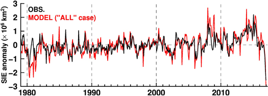
Figure 1. Time series of monthly Antarctic sea ice extent anomalies from 1979 to 2016 (black: observation and red: numerical model). The anomalies are calculated by subtracting the monthly climatology from the sea ice extent for the period 1979–2016. Correlation coefficients between the two with and without the linear trends are 0.74 and 0.69, respectively. The 99% significant level (n = 444) is at r = 0.123.
Download figure:
Standard image High-resolution image
Figure 2. Seasonal anomaly maps of (a)–(d) observed sea ice concentration and SST, (e)–(f) atmospheric variables at the 925 hPa surface, and (i)–(l) modeled sea ice concentration and SST in 2016. These anomalies are calculated by subtracting the climatology averaged over 1979–2016 from the 2016 fields. The atmospheric variables are air temperature (color), wind (vector), and geopotential height (colored contour with 10 m interval). Black and green lines in panels (a)–(d) and (i)–(l) show the sea ice edges in 2016 and the climatology, respectively.
Download figure:
Standard image High-resolution image3.1. Total SIE anomaly
Here we show results from the additional three experiments ('THD + DYN', 'INI + THD', and 'INI + DYN' series) to examine the sea ice response to changes in the initial sea-ice and oceanic conditions at the beginning of the year, thermodynamic surface forcing, and wind stress. The monthly time series of the ensemble mean of the total SIE anomaly in the numerical experiments, as well as the 'ALL' case, are shown in figure 3. Details of the numerical experiments and the SIE anomaly at December (the end of integration) are summarized in table 1.

Figure 3. Time series of total sea ice extent anomaly in the numerical experiments (red: 'ALL' case, purple: 'THD + DYN' series, green: 'INI + THD' series, and blue: 'INI + DYN' series). Dots show results for the ensemble members and colored lines show the ensemble mean. Error bars show one standard deviation, showing the ensemble spread. The anomaly in the 'THD + DYN', 'INI + THD', and 'INI + DYN' series are calculated by subtracting the 'ALL'-case seasonal climatology (1979–2016) from the sea ice extent.
Download figure:
Standard image High-resolution imageThe temporal evolution in the 'THD + DYN' series is very similar to that in the 'ALL' case (figure 3(a)), but the ensemble mean anomaly at the end of the integration (December) in the 'THD + DYN' series case is higher than that in the 'ALL'. This result indicates that thermodynamic surface forcing and wind stress are mainly responsible for the time evolution of the total SIE anomaly and that the combination of sea-ice and oceanic conditions from the previous summer (1 January) contributed, to some extent, to the total SIE anomaly at the end of the year.
The temporal evolution of the ensemble mean total SIE anomaly in the 'INI + THD' series is similar to that in the 'ALL' case throughout the year (figure 3(b)). However, the spring reduction of the ensemble mean total extent anomaly in the 'INI + THD' series is less than that in the 'ALL' case. This result suggests that thermodynamic forcing in 2016 cannot fully explain the spring reduction. The ensemble mean time series in the 'INI + DYN' series is different from the 2016 extent anomaly in the 'ALL' case but is stable just above zero-anomaly until October (figure 3(c)). The time series in the 'INI + DYN' series and the 'ALL' case show a substantial decline in the last few months (from October/November to December). The final two-/three-month reduction in SIE in the 'INI + DYN' series indicates that, in 2016, the wind stress amplified the springtime reduction. The comparison of results from the 'ALL' case and the 'INI + THD'/'INI + DYN ' series suggests that thermodynamic surface forcing is mainly responsible for the total SIE anomaly through 2016 and that wind stress substantially modified it in the spring season.
The difference between the December total SIE anomaly in each ensemble mean of three experiments and the 'ALL' case (6th column in table 1) can be used to estimate the relative contributions of these factors to the 2016 SIE minimum in the model. We estimate the contribution of thermodynamic forcing to be 53% from the difference between the 'ALL' case and 'INI + DYN' series (1.71 × 10⁶ km2) from the sum of the anomalies (3.24 × 10⁶ km2), assuming linearity in the responses. In the same way, the wind stress and the initial conditions account for 34% and 13% of the 2016 SIE minimum in spring, respectively.
3.2. Regional distributions of SIC and SST anomalies
Next, we examine the atmospheric factors responsible for the regional patterns of sea ice decreases in the 2016 spring (when the total SIE was minimum) by comparing results from the numerical experiments. Three negative and three positive SIC anomalies are identified near the sea ice edge region in both the satellite observations and the 'ALL' case (figures 2(d), (l), and 4(a)). The total areal extent of the negative anomalies is much larger than that of the positive anomalies, resulting in the pronounced negative total SIE anomaly (figure 1). The negative SIC anomalies near the sea ice edge are found in longitude ranges of 110°W–30°W (Bellingshausen Seas to the western Weddell Sea), 25°E–80°E (south eastern Indian Ocean), and 120°E–160°W (the western Pacific Ocean to the Ross Sea), separated by the positive anomalies. The SST anomalies also have a wavenumber-3 pattern. As shown in figures 2(d) and (l), the spatial anomaly patterns of the spring sea ice edge and SST in the 'ALL' case are consistent with the observed ones.
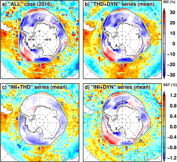
Figure 4. Anomaly maps of modeled sea ice concentration and SST in spring (October–December) in the numerical experiments (a): 'ALL' case, (b): 'THD + DYN' series, (c): 'INI + THD' series, and (d): 'INIT + DYN' series. The maps in (b)–(d) are ensemble mean of the experiments. These anomalies are calculated in each case by subtracting the climatology in the 'ALL' case (1979–2016) from the field. Black and green contours show the sea ice edges in 2016 and the climatology, respectively. Uppercase letters A–E demarcate zones of sea ice reduction near sea ice edge regions, and lowercase letters x–z the ice-pack regions.
Download figure:
Standard image High-resolution image
We classify the negative anomalies near the sea ice edge into five regions, and label them with upper cases (A, B, C, D, and E in figure 4(a)). Similarly, other negative anomalies within the pack-ice regions are labeled with lower cases (x, y, and z). The modeled negative anomalies in the pack-ice region are present in longitude range of 20°W–15°E (labeled with 'x', a coastal region in the central Weddell Sea), 65°E–90°E (labeled with 'y', off Cape Darnley and Prydz Bay), and 180°−135°W (labeled with 'z', off Marie Byrd Land). Looking at the SST anomalies in the 'ALL' case (figure 4(a)), the positive (warmer) anomaly regions roughly correspond with most regions of the negative SIC anomaly regions near the sea ice edge (e.g., the labeled regions of A, C, D, and E).
The anomalies of SIC and SST in the ensemble mean of the 'THD + DYN' series are almost the same in the 'ALL' case (figures 4(a) and (b)), except for the areal extent of the negative anomaly in the coastal Weddell Sea (region x). This result indicates that surface boundary conditions (the combination of wind stress and thermodynamic forcing) are mainly responsible for the anomaly patterns in the 2016 spring minimum.
The ensemble mean of 'INI + THD' series, whose pattern is considered to come from thermodynamic forcing (figure 4(c)), produces the springtime negative SIC anomalies in the outer-pack regions of A, C, and E but does not reproduce those in the Weddell Sea and the western Pacific Ocean (regions B and D). The spatial pattern of SIC in the inner pack-ice region for the 'INI + THD' series is quite different from those in the 'ALL' case and the 'THD + DYN' ensemble mean (figures 4(a)–(c)). The SST anomalies in 'INI + THD' series, on the other hand, are similar to those in the 'ALL' case and the 'THD + DYN' ensemble mean, but with a smaller amplitude of anomalies. These results suggest that thermodynamic surface forcing associated with atmospheric circulation change is responsible for the broad observed regional negative SIC anomalies in the 2016 sea ice edge, except for the western Weddell Sea and western Pacific Ocean sectors, and the broad SST anomaly fields around the entire Southern Ocean.
A comparison of the SIC anomaly patterns in the ensemble mean of the 'INI + DYN' series with the 'ALL' case and the 'THD + DYN' ensemble mean (figures 4(a), (b) and (d)) demonstrates that in 2016 the wind stress is largely responsible for the sea ice edge retreat in the Weddell (B), the western Pacific Ocean (D), and Ross Sea (E) regions, and the reduction in the pack-ice regions (x, y, and z). Similarly, the wind stress explains the sea ice advance (positive SIC anomalies near the sea-ice edge) in the regions around 0° and 135°W. There is strong similarity in the large-scale pattern in the pack-ice region anomaly between the 'INI + DYN' ensemble mean and the 'ALL' case/'THD + DYN' ensemble mean, indicating that wind stress controls sea ice distribution there. The SST anomalies in the 'INI + DYN' series are entirely different from those in the 'ALL' case/'THD + DYN' ensemble mean and observations, except for the western Pacific Ocean where wind stress plays a role in the regional SST pattern. This again indicates that the large-scale patterns in SST anomalies over the Southern Ocean are explained by thermodynamic surface forcing, not by wind stress.
4. Summary and discussion
We have investigated key factors responsible for the extraordinary 2016 Antarctic sea ice minimum, based on analyses of atmospheric re-analysis data and results from a coupled ocean-sea ice model. Atmospheric conditions over the Southern Ocean changed dramatically through 2016, from westerly wind and cold air temperature anomalies in summer (JFM) to easterly wind and warm anomaly conditions in the following spring (figures 2(e)–(h) and the supplementary material S2). The change in the wind pattern corresponds to a pronounced shift from positive to negative phases of SAM. In the intervening period (autumn and winter), a wavy structure in the atmospheric circulation developed and associated northerly winds effectively transported warmer air poleward. Our ocean-sea ice model driven by atmospheric surface boundary conditions calculated from the ERA-Interim dataset satisfactorily reproduced the time series of observed Antarctic SIE from 1979 to 2016 (figure 1) and the regional anomalies of SIC in 2016 (figures 2(a)–(d) and (i)–(l)).
We have estimated, from a series of numerical experiments, the relative contributions of (i) thermodynamic surface forcing, (ii) wind stress, and (iii) the previous summer's sea-ice and oceanic conditions to the 2016 sea ice minimum (table 1 and figure 3). All components were primed to reduce Antarctic sea ice, e.g., warmer air, eastward wind anomalies leading to a southward anomaly of Ekman sea ice drift, and less sea ice and cooler SST at the beginning of 2016. Thermodynamic surface forcing and wind stress explain 53% and 34% of the reduction in the total SIE in the 'ALL' case, respectively, and the previous summer sea-ice and oceanic conditions are non-negligible (13%), confirming the general findings of previous studies (Stammerjohn et al 2008, Holland et al 2013) that advance in one season is partially related to the retreat in the previous season.
We further examined the factors responsible for the regional SIC anomaly pattern (figure 4). It was found that the warm circumpolar conditions reduced the overall SIC near the sea ice edge region, except in the Weddell Sea and the western Pacific Ocean where wind stress plays an important role in sea ice edge retreat. Furthermore, the model suggested that changes in wind stress contributed to SIC reduction in the inner pack-ice regions (which is not strongly reflected on the overall SIE). Note that while our experiments demonstrate the importance of thermodynamic forcing, we could not separate atmospheric and oceanic contributions. As well as atmospheric warming, rapid southward migrations of the observed/modeled warm SST anomaly (which is also mainly caused by atmospheric warming (figure 4)) likely contributed to the 2016 Antarctic sea ice minimum (figures 2 and 4) through ocean melting as discussed in Reid et al (2017) and Stuecker et al (2017). Stuecker et al (2017) showed that atmospheric modes, such as ENSO and SAM, have a large impact on the 2016 Antarctic sea ice fields. Changes in these modes (i.e., atmospheric circulation changes) have influenced the sea ice fields through changes in wind stress and thermodynamic fluxes, and thus this study is complementary to their study.
Antarctic SIE has shown a modest increase in the modern satellite era after 1979 (Parkinson and Cavalieri 2012, Comiso et al 2017, de Santis et al 2017). The causes of the positive trend have been actively discussed in the literature: e.g., wind stress (Holland and Kwok 2012, Holland et al 2014, Zhang 2014, Matear et al 2015, Meehl et al 2016), thermodynamic forcing (Liu et al 2004, Lefebvre and Goosse 2008, Turner and Overland 2009, Hobbs and Raphael 2010, Fan et al 2014, Massonnet et al 2015, Kusahara et al 2017), ocean temperature (Jacobs and Comiso 1997, Meredith and King 2005), freshwater input from the Antarctic Ice Sheet (Bintanja et al 2013), and so on. This discussion about drivers of sea ice trends was further summarized in Hobbs et al (2016). A recent study by Comiso et al (2017), from a combined analysis of updated SIC data and re-analysis air temperature data, suggests that atmospheric cooling over the Southern Ocean, as part of the regional variability in global warming, drives the positive trend in the Antarctic sea ice. Similarly, consistent cooling signals are also found in SST over the Southern Ocean (Fan et al 2014). The SAM (the major atmospheric mode in the Southern Hemisphere) has shifted to a more positive phase in recent decades (Abram et al 2014) and the stronger westerly winds associated with deepening of geopotential height over the Antarctic continent has steepened the atmospheric temperature gradient between southern high and low latitudes, resulting in atmospheric cooling trend over the Southern Ocean.
Climate models predict that global warming will be accompanied by a stable decline in Antarctic SIE over the 21st century (Bracegirdle et al 2008). For many climate models that failed to reproduce the recent positive trend in Antarctic sea ice over the recent decades, the decline was predicted to have already begun (Shu et al 2015, Schneider and Deser 2018), and this may be partially explained by the large difference in the representation of SAM in the models (Zheng et al 2013). Several numerical models driven by specified atmosphere conditions from re-analysis data (Holland et al 2014, Zhang 2014, Massonnet et al 2015, Kusahara et al 2017) can capture the observed positive sea ice trend to some extent. These results suggest that sea ice models can fundamentally reproduce and predict Antarctic sea ice behavior to some extent, if the correct atmospheric conditions are given.
A turning point of Antarctic sea ice from the recent modest increasing trend to a decreasing trend will occur if the ongoing global warming signal dominates the cooling effect with a positive shift in SAM. The SAM index changed to a negative phase in 2016, and then relative heat waves from subtropical regions propagated to southern high latitudes (figures 2(e)–(h)), resulting in the record-breaking Antarctic sea ice minimum (Reid et al 2017, Stuecker et al 2017, Turner et al 2017, Schlosser et al 2018). Our study confirms that in addition to continuous remote-sensing observations of Antarctic sea ice, ongoing monitoring of atmosphere and ocean conditions over the entire Southern Hemisphere (i.e., the ocean-atmosphere interaction between polar and subtropical regions (Meehl et al 2016, Stuecker et al 2017)) is required to better understand and predict upcoming changes and variability in Antarctic sea ice.
Acknowledgments
This research was supported by the Australian Government's Cooperative Research Centre through the ACE CRC, and contributes to ACE CRC Project R1.3 and AAS Project 4116. GW was supported by the Australian Research Council's Future Fellowship program. HH was supported by JSPS KAKENHI Grant Number 26247080. We thank two anonymous reviewers for their careful reading and helpful comments on the manuscript.
The data used in the analysis and model configuration were acquired from the following websites: sea ice concentration: ftp://sidads.colorado.edu/pub/DATASETS/nsidc0051_gsfc_nasateam_seaice. RTopo1 for bottom topography and draft: https://doi.pangaea.de/10.1594/PANGAEA.741917. PHC for initial and lateral boundary conditions: http://psc.apl.washington.edu/nonwp_projects/PHC/Climatology.html. The climatological surface boundary forcing data: http://omip.zmaw.de/. ERA-Interim for inter-annual surface boundary forcing for the period 1979–2016: http://ecmwf.int/en/research/climate-reanalysis/era-interim.