


Abstract
While the global carbon budget (GCB) is relatively well constrained over the last decades of the 20th century [1], observations and reconstructions of atmospheric CO2 growth rate present large discrepancies during the earlier periods [2]. The large uncertainty in GCB has been attributed to the land biosphere, although it is not clear whether the gaps between observations and reconstructions are mainly because land-surface models (LSMs) underestimate inter-annual to decadal variability in natural ecosystems, or due to inaccuracies in land-use change reconstructions.
As Eurasia encompasses about 15% of the terrestrial surface, 20% of the global soil organic carbon pool and constitutes a large CO2 sink, we evaluate the potential contribution of natural and human-driven processes to induce large anomalies in the biospheric CO2 fluxes in the early 20th century. We use an LSM specifically developed for high-latitudes, that correctly simulates Eurasian C-stocks and fluxes from observational records [3], in order to evaluate the sensitivity of the Eurasian sink to the strong high-latitude warming occurring between 1930 and 1950. We show that the LSM with improved high-latitude phenology, hydrology and soil processes, contrary to the group of LSMs in [2], is able to represent enhanced vegetation growth linked to boreal spring warming, consistent with tree-ring time-series [4]. By compiling a dataset of annual agricultural area in the Former Soviet Union that better reflects changes in cropland area linked with socio-economic fluctuations during the early 20th century, we show that land-abadonment during periods of crisis and war may result in reduced CO2 emissions from land-use change (44%–78% lower) detectable at decadal time-scales.
Our study points to key processes that may need to be improved in LSMs and LUC datasets in order to better represent decadal variability in the land CO2 sink, and to better constrain the GCB during the pre-observational record.
Export citation and abstract BibTeX RIS

Original content from this work may be used under the terms of the Creative Commons Attribution 3.0 licence.
Any further distribution of this work must maintain attribution to the author(s) and the title of the work, journal citation and DOI.
1. Introduction
Changes in atmospheric CO2 growth rate can either be measured directly from atmospheric composition measurements (following 1959) or from ice-core records (earlier periods) [5]. Alternatively, they can be reconstructed from the balance of sources (fossil fuel burning and land-use change emissions) and sinks (ocean and natural terrestrial ecosystems) [1]. The latter approach allows understanding the processes influencing atmospheric CO2 changes, but requires accurate estimates of each term of the global carbon budget (GCB). Over the 20th century (20 C), the mismatch between observed atmospheric CO2 growth rate and state-of-the-art reconstructions of anthropogenic emissions and natural sinks varies considerably. The budget gap is small during the observational period, but considerably large during the mid-1920s to mid-1930s and especially between 1940 and the mid-1950s [1, 2]. The reasons for such budget gaps may differ depending on the period considered, but are most likely due to (i) the systematic underestimation by land-surface models (LSMs) of inter-annual variability in the natural terrestrial sink and (ii) the high uncertainty in land-use change (LUC) estimates [2].
During the 1940s, atmospheric CO2 concentrations stabilized, without a clear process having been so far identified [2]: the sink calculated from current land and ocean models is 0.9–2 Pg C . yr−1 lower than the sink needed to balance CO2 sources at the time. Decadal changes in the ocean sink alone likely do not explain more than 0.5 Pg C . yr−1, implying a sink gap in the land biosphere of 0.4–1.5 Pg C . yr−1. Bastos et al [2] proposed two main processes influencing uncertainty in reconstructions in this period: (i) enhanced vegetation growth in response to high-latitude warming not fully captured by LSMs and (ii) natural vegetation expansion following cropland abandonment during the second World War (WWII) period, not accounted for in current LUC datasets. Additional processes could further contribute to enhance the terrestrial sink in the 1940s: e.g. an initial response of ecosystems to increased nutrient deposition from fossil-fuel burning, or decrease in wood-harvest due to demographic changes [2].
Pinning-down the origin of such mismatches for the pre-observational period is challenging, since there are virtually no measurements of natural carbon stocks, and information about LUC, if existing, is hard to compile and harmonize at the global scale. The integration of nutrient cycles in LSMs is still a challenge, and most models do not simulate explicitly the effect of wood-harvest on forest carbon stocks. However, insights might be obtained about the sources of uncertainty in the earlier 20 C carbon budget by focusing on key regions and processes. Here we evaluate the potential contribution of the two main processes discussed in Bastos et al [2]—high-latitude warming and land-abandonment—to explain the gap sink in the early 20 C. In this context, northern Eurasia is a region of particular interest, covering about 15% of the terrestrial surface, accounting for a significant fraction of the global terrestrial sink (0.3–1.4 Pg C .yr−1 in 1985–2008 [8]), and 20% of the global soil organic carbon pool [9]).
The warming over land between the mid-1930s until ca. 1950 is a robust feature of the global temperature record [10, 11], reproduced by models [12], observed in tree-ring and oxygen isotope proxies [13, 4, 14], and associated with faster glacier retreat [15, 16]. According to high-latitude (>60°N) station data [17], North Atlantic circulation promoted very warm conditions during the 1930s and 1940s (2 °C–3 °C above the 1961-90 mean) between autumn and spring, with strong anomalies covering western Russia, the Ural region and extending to the central Siberian Plateau. Such early-season warming could have promoted vegetation growth by advancing the growing season and enhancing photosynthesis, explaining the increase in tree-ring width reported in Eurasian sites by D'Arrigo et al [4].
Reconstructions of LUC emissions (ELUC), including those from TRENDYv4 models [2, 6, 18], commonly apply LUC datasets from [19] (HYDE 3.1) and [26] (LUH1, itself based on HYDE 3.1). These are based on UN Food and Agricultural Organisation statistics (FAOSTAT) of country-level agricultural area data after 1961. Before 1961, cropland statistics from national literature exist only for some countries and are thus hard to compile and harmonize in a global product. In order to ensure consistency between countries, HYDE 3.1 extrapolate country-level agricultural area backwards using country–level total population and cropland area per-capita ratios. This assumption may be unrealistic for certain periods in history, as demographic and economic changes may influence cropland per capita ratios or introduce variability in LUC, and hence in ELUC.
The population in Eurasia in the first half of the 20th century was highly rural. In the Former Soviet Union (FSU), only 18% of the population lived in cities in 1926 (33% in 1939) and agriculture was a key economic sector. In 1927–28, agricultural output contributed 42% of gross FSU production (industry and agriculture combined) [21]. This period was marked by several major food crisis, resulting from a combination of recurring droughts and drastic political and economic changes, with severe impacts on population [20]. The Russian Revolution and the Civil War have been linked to a decrease in grain output of ca. 40% between 1913 and 1920 [21]. Two massive famines occurred in 1921–22 and 1932–33, affecting millions of people. Not only did these famines and the successive political crises result in increased mortality, they also led to massive population migrations [22]. The 1930s further registered a massive transition from small privately-owned farms to collective property of large farms. During the first years of the collectivization period (1929–1931) roughly 1.5 million people were estimated to have been deported [21]. Of all crises affecting FSU during the early 20 C, WWII had arguably the most dramatic impacts. The war was responsible for the death of 26.6 million people (14% of the population) [23], and for the evacuation of at least 10 million people from the western front, where most agricultural area was located [24]. During the war years, massive land-abandonment due to mortality and migration and a decrease in agricultural production of 40% (against an 8% decrease in industrial production) have been reported, with peak reduction by 50%–69% in 1943 compared to 1940 [24, 21, 25]. Given such drastic economic and demographic changes, the relationship between total population and crop area likely changed over the 20 C, rather than being approximately constant as defined in HYDE 3.1.
In order to better characterize the physical and carbon cycling processes in northern Eurasia, we use an LSM with improved representation of high-latitude hydrology, soil carbon dynamics and phenology (ORCHIDEE-MICT v8.4.1 [3]) that was shown to reproduce the amount of soil carbon in the high-latitudes and the seasonal exchange of CO2 in recent decades. On a second step, we compare cropland area statistics from LUH1 with annual values of agricultural area in the FSU from official Russian Empire (during the pre-Soviet period, 1913–1916) and Soviet statistics between 1917 and 1961. We evaluate whether the datasets capture the socio-economic changes in FSU prior to 1961 by comparing them with demographic and economic statistics. Finally, we derive land-cover maps based on the new cropland data to calculate the resulting ELUC over Eurasia in the early 20 C. We compare our new estimates of C-sequestration by natural ecosystems and ELUC with the ones from TRENDYv4 LSMs [2, 6, 18, ] in order to understand if an improved description of soil-C and phenology in high-latitudes by LSMs and the use of country-level land-use statistics prior to 1961 might contribute to explain the gap between observations and GCB reconstructions in [2].
2. Data and methods
2.1. Climate data
The CRU/NCEP v5.4 dataset, used to force models in TRENDYv4 [2, 6, 18], provides 6 hourly data of air-surface temperature, rain and snowfall, surface radiation and air specific humidity over 1901–1999 at 0.5°spatial resolution. For comparability with TRENDYv4, we used CRU/NCEP v5.4 in our analysis and as forcing of ORCHIDEE-MICT simulations.
2.2. Reference LUC dataset
The LUH1 [26] is a state-of-the-art dataset used to force LSMs in several GCB studies [2, 6, 18]. LUH1 provides annual values of fractional cover and transitions of cropland, pasture, and primary and secondary vegetation, at 0.5 × 0.5 degree lat/lon from 1500 until 2100. Cropland, pasture, urban, and ice/water fractions between 1500 and 2005 are based on the HYDE 3.1 database [19] that provides gridded time series of historical population and land-use for the Holocene. HYDE3.1 values are based on national statistics compiled by FAOSTAT [27] from 1961 onwards, and calculated from cropland per capita ratios (varying little) combined with national population statistics prior to 1961.
Forest, crop and grassland fractional cover and transitions data from LUH1 were used to produce 2 × 2 degree lat/lon maps of the 13 plant functional types (PFTs) from ORCHIDEE-MICT, following the method in [28]. These PFTs consist of bare soil, eight forest PFTs, two crop PFTs (C3 and C4 crops) and two grass PFTs (C3 and C4 grass). Since ORCHIDEE-MICT does not explicitly simulate grazing and pasture management, pastures are treated as natural grassland. Henceforth, we refer to this dataset simply as LUREF. It should be noted that small differences between the original LUH1 and LUREF are expected due to the conversion to PFTs and to a coarser grid. Since we perform a sensitivity study by comparing pairs of simulations, these differences should not significantly affect the results. The geographical distributions of forest, grassland and cropland over the 20 C in FSU are shown in figure S1.
2.3. Official statistics of the FSU
For certain countries, such as the FSU, national land-use statistics are available before 1961. We collected annual cropland area reported in official books of statistics from the State Statistics Bureau (GOSKOMSTAT), responsible for compiling economic and demographic data (incuding the ones used by FAOSTAT for subsequent years). We collected and harmonized cropland area statistics prior to 1961 for the Russian Empire during the pre-Soviet period (1913–1917) and for the FSU between 1917 and 1961 by GOSKOMSTAT. Official data for 1941–1945 was compiled in 1959, but only became declassified in 1990 by the end of the Perestroika [29], allowing to evaluate the impact of WWII in ELUC in northern Eurasia. The data was likely originally collected at oblast level (administrative units roughly comparable to states or provinces), but official records provide aggregated values by country (former Soviet Republics) or the FSU total.
We produced new PFT maps by combining spatial patterns from LUREF with the changes in total crop area in FSU from GOSKOMSTAT, analogous to other modelling studies [38]. A step-by-step description of the conversion from national totals to spatially-explicit maps is provided in supplementary methods available at stacks.iop.org/ERL/13/065014/mmedia. This dataset is hereafter referred to as LUNEW.
Population and economic statistics provide useful proxies to evaluate the variability of crop area in LUREF and LUNEW. We collected population information reported by the GOSKOMSTAT for the same period of LUNEW (supplementary data). National statistics provide FSU population totals and discriminate between urban and rural population based on the designation of permanent residence. This does not necessarily mean population working in agriculture, and data further have a gap during 1940–1945, when LUNEW reports a big cropland drop. We collected additionally active population data (i.e. population ensuring the supply of labour for the production of economic goods and services) from the GOSKOMSTAT between 1913 and 1961, which presents several gaps but covers the period 1940–1945. Finally, we compared population statistics with economic data [30, 31].
2.4. ORCHIDEE-MICT simulations
ORCHIDEE is a global LSM [32] representing the main energy, hydrological and carbon cycling processes in land ecosystems. The ORCHIDEE-MICT v8.4.1 includes an enhanced description of high-latitude hydrology, the effect of snowpack insulation in winter in soil temperature, and an improved description of interactions between soil freeze, soil water holding capacity and thermic conductivity described in [33, 3]. Fire occurrence is simulated using the SPITFIRE fire model as described in [34], which has been shown to simulate boreal fires consistent with historical reconstructions [35]. For crop PFTs, 85% of NPP is harvested and consumed directly [36]—and therefore most C is not returned to the soil. Crop PFT parameters related with photosynthesis were adjusted to reproduce earlier 20 C crop productivity (table S1, figure S2). Grassland parameterization here follows the one proposed by [37]. Since we do not have any information that could allow producing gross LU transition maps, ELUC are calculated from the net difference in the land-use/land-cover class fraction between two consecutive years [36]. Although our focus is the early 20 C, we extend the simulations up to the end of the century in order to evaluate the simulated C-stocks against observation-based data.
We ran five factorial simulations to test the sensitivity of C-stocks and fluxes to climate variability and to different LUC scenarios, summarized in table 1. In order to ensure comparability with values in [2], we follow the protocol from TRENDYv4 [18] for the baseline simulation (SRef): ORCHIDEE-MICT is forced with historical climate between 1901 and 1999 and prescribed LUC from LUREF. However, here we focus on the northern Eurasian region, in particular on the territory corresponding to LUNEW (figure S1).
Table 1. Summary of the ORCHIDEE-MICT factorial simulations performed in this work and the corresponding processes to be tested by each simulation. In SClim, the climate forcing is cycled over the same 10 yr period as the one used for the spinup (1901–1910). All simulations are forced with historical atmospheric CO2 concentrations from observations.
| Simulation | Climate | LU map | Test |
|---|---|---|---|
| SRef | Historical | FSUREF | — |
| SClim | Cyclic | FSUREF | Climate |
| SnoLUC | Historical | FSUREF 1860 | ELUC |
| SFOR | Historical | FSUNEW FOR | FSUNEW crop → Forest |
| SGRA | Historical | FSUNEW GRA | FSUNEW crop → Grassland |
To test the sensitivity of ELUC to the two LUC datasets, we ran three additional simulations: one with fixed pre-industrial (1860) land-cover map from LUNEW, i.e. no land-use (SnoLUC), and other two simulations where cropland is prescribed from LUNEW. We define two extreme scenarios for the range of forest vs. grassland trajectories following land-abandonment: FOR and GRA, corresponding to forest or grassland PFTs being preferentially assigned to the fraction of cropland removed (figure S3, SFOR and SGRA, respectively). All three simulations were forced with historical climate. To evaluate the contribution of climate anomalies to the simulated CO2 fluxes, an additional simulation was performed with 1901–1910 cyclic climate (SClim).
3. Results and discussion
3.1. Natural climate variability
Temperature from CRU/NCEP indicates the occurrence of a warming event in Eurasia above 60°N from the mid-1920s until the mid-1950s (figure 1(a)). A strong peak is observed between ca. 1935–1945, with temperatures 0.5 °C above the reference mean (1901–1930), only matched after the mid-1980s when anthropogenic global warming started to have a clear fingerprint on regional temperature. Both TRENDYv4 and SRef simulations (figure 1(b)) show the characteristic increasing trend of net biome production (NBP) over the 20 C and SRef values are generally within the TRENDYv4 inter-model range, except for few years during the mid-1920s, around 1930, and for a long period starting in the late 1930s and lasting until the mid-1950s. These differences coincide with the high-latitude warming events shown in figure 1, excepting 1980–1999 In this period widespread warming is observed but NBP from SRef is very close to the TRENDYv4 inter-model mean, pointing to different driving processes than in the earlier events. NBP simulated by SClim is generally within TRENDYv4 inter-model range, but does not reveal significant NBP changes during the periods when SRef and TRENDYv4 diverge. Therefore, the strong sink during the 1920s and 1940s can be mainly attributed to the high-latitude warming episodes induced by decadal atmospheric circulation variability [17].

Figure 1. Warming episodes in Eurasia (FSU territory, figure S1) over the 20 C and resulting impacts on CO2 uptake by ecosystems (NBP, counted positively for a carbon gain by land ecosystems). (a) Latitudinal distribution of average annual temperature anomalies (from CRU/NCEP) over Eurasia. Anomalies are calculated relative to the 1901–1930 mean. (b) Simulated terrestrial CO2 uptake (NBP) in Eurasia between 1900–1999, simulated by the set of models from the TRENDYv4 intercomparison [18] (bold black line indicated inter-model median and thin lines the range) and by SRef (red) and SClim (blue). In (b) the horizontal bar highlights the years when average temperature anomaly over the whole territory is above 0.1 °C.
Download figure:
Standard image High-resolution imageLarger discrepancies are found during the 1940s decade, when SRef indicates strong C-sequestration in Eurasian ecosystems of 0.6 Pg C . yr−1 (figure 1), while TRENDYv4 models indicate a difference one order of magnitude lower (0.04 Pg C . yr−1). We analyse this period in more detail, as it coincides with discrepancies in the GCB reconstructions [2]. As shown in figure 2(a), the 1940s were considerably warmer than the previous decade over most of Eurasia, particularly during Mar-May in the latitude band between 55–75oN. Warming was also registered in summer, although much weaker than in spring. SRef simulates NBP 13 gC . m−2 . yr−1 higher than the previous decade's mean, mostly within the latitude band coinciding with warming (figure 2(b)), while SClim indicates a negligible difference between the two decades (1 gC . m−2 . yr−1). The combination of very warm springs with mild summers favours increased gross primary productivity due to earlier onset of the growing season (figure S4(a) and (b)), while keeping heterotrophic respiration close to average (figure S4(c)). At the same time, in high-latitudes (above 60oN), vegetation growth is limited by access to deep water in permafrost soils. The model simulates a deepening of the active layer thickness in the permafrost regions in response to the 1940s warming (figure S5), promoting higher soil-water availability to support vegetation growth. These conditions combined favour a strong climate-related peak of vegetation growth during the early 1940s (figure S6), and subsequent accumulation of C in the soils, leading to an enhanced C-sink.

Figure 2. Latitudinal differences between the 1940–1949 and 1930–1939 over the FSU region, for (a) surface temperature from CRU/NCEP, (b) net CO2 uptake (NBP), (c) carbon stocks in vegetation and (d) in soil. The two simulations with historical (SRef, in red) and cyclic (SClim, in blue) climate variability are compared with the corresponding variables from the TRENDY models (shown individually in thin grey lines). The number labels correspond to the sum of the latitudinal anomalies for SRef (red) and SClim (blue) in the corresponding units.
Download figure:
Standard image High-resolution imageSimulated C accumulation in FSU vegetation and soils in the 1940s is 59 gC . m−2 and 64 gC . m−2 higher than in the previous decade respectively, mainly coinciding with warm anomalies (figures 2(c) and (d)). Vegetation growth peaks at higher latitudes than temperature, because ecosystems in high-latitudes are strongly energy limited, and therefore more sensitive to temperature and to the increased water availability in permafrost regions. Changes in vegetation C simulated by TRENDYv4 also show an increase in high-latitudes, even though smaller than in SRef. SRef simulates lower soil-C accumulation during the 1940s than SClim due to the warming impact on respiration. The stronger increase in soil input from litterfall than the change in decomposition rates explains the increase in soil-C during the 1940s.
TRENDYv4 models also simulate a small increase of NBP coinciding with warming but only in latitudes below 60°N, and estimate very little change in vegetation and soil-C. This is likely because most models do not explicitly simulate permafrost dynamics or vegetation growth limitations due to soil freezing and lack the coupling between soil temperature, hydrology and carbon, contrary to ORCHIDEE-MICT as discussed previously. ORCHIDEE-MICT results are further consistent with increased tree-ring width during the 1930s and 1940s in high-latitude locations in Eurasia reported by [4]. These differences could explain ca. 60% of the additional sink required in [2], considering the gap of 0.7 Pg C. yr−1 estimated by LSMs in the 1940s.
3.2. LUC and resulting emissions
Figure 3(a) compares cropland area from LUREF and LUNEW with total and active population data. LUREF (bold line, black) estimates systematically higher cropland area than LUNEW (black line, + markers) but is also much less variable. LUREF is based on HYDE3.1, that reconstructed cropland from total population (red line) and captures mainly decadal variations. On the contrary, active population (red line, + markers) presents large variations, increasing during the 1930s until 1940, followed by a sharp drop of about 30% between 1940 and 1942.
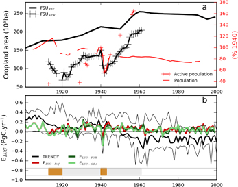
Figure 3. Cropland area reconstructions and corresponding LUC emissions. (a) Agricultural area in the FSU in the two datasets used here: FSUREF (bold black line) and FSUNEW (black line with markers). For comparison, we show the total and active population collected from national statistics (red, from supplementary data). The left yy-axis refers to the two agricultural extent datasets, while the right yy-axis refers to the population values, which are presented as % of the 1940 reference value.(b) ELUC simulated by ORCHIDEE-MICT and by the TRENDYv4 models [18] (bold black curve represents the inter-model mean and the shade the inter-model spread), which are used as reference values in [2]. The horizontal bar indicates the period of FSUNEW and the corresponding periods of strong decrease in cropland area (dark yellow).
Download figure:
Standard image High-resolution imageVariations in cropland area reported by GOSKOMSTAT (LUNEW) reflect the fluctuations in crop area due to the main major socio-economic disruptions happening in the first half of the 20 C: Russian participation in World War I (1914–1917) and the Russian revolution (1917, data are missing for 1918 and 1919), the 1921–22 famine and the WWII period. The 1930s crisis is reflected in our data by a slight decrease in cropland area between 1930 and 1932 followed by a stagnation until 1940. The sharp drop in total cropland area between 1940 and 1942 in LUNEW corresponds mainly to a massive cropland abandonement in occupied and contiguous regions (that dropped from ca. 71 Mha in 1940 to 23 Mha (−68%) in 1943, supplementary data), consistent with previous reports [21, 24] and with active population and GDP variations (figures 3(a), S7). On the contrary, LUREF does not capture these short-term variations, reporting an increase in cropland extent during the 1920s and 1930s, and only a slight decrease during the 1940s. This implies that using total population to extrapolate country-level crop area (as used in [19]) may miss important LUC changes, by not reflecting the effects of migratory fluxes between rural and urban areas (which are highly relevant in the early 20 C), nor variations in active work force due to war (or other disrupting events), nor the mobilization of labour to other sectors of the economy [24]. Nevertheless, it should be noted that using total population data may still be the best variable to consistently harmonize country-level data at global scale for earlier periods in history, when other indicators may not be available.
Emissions from LUC calculated using LUREF map (ELUC-Ref obtained by the difference between SRef and SnoLUC) remain within the range of TRENDYv4 models (S2–S3) during the 20 C (figure 3(b)). While the TRENDYv4 inter-model mean indicates an increasing sink due to LUC over the century (negative trend) in FSU, ORCHIDEE-MICT simulates a small but relatively stable LUC source. A strong decrease in ELUC is simulated by ORCHIDEE-MICT between 1901 and 1915, contemporary with grassland expansion (figure S3). This decrease is also reported by the TRENDYv4 inter-model mean, although less pronounced. From 1920 until the mid 1950s, ELUC-Ref remain close to the TRENDYv4 inter-model mean.
The two simulations forced with LUNEW (SFOR and SGRA) do not lead to remarkable differences in ELUC as compared to the reference simulation, except between 1913 and 1920 and during 1940–1945. Both periods coincide with the strong decreases in cropland extent reported in LUNEW and are associated with C accumulation in biomass and soils starting in 1922 and peaking in the first years of the 1940s. In spite of a concurrent enhancement of respiration, increased vegetation growth results in fast C accumulation in biomass and soils. An increase in biomass C is simulated in the 1920–1930 (+0.1 Pg C . yr−1), although the one in the 1940s is stronger (+0.4 Pg C . yr−1) and sustained for longer. The 1920s strong C-sink may be related to the forest area expansion between 1910 and 1920 (also present in SRef), combined with the effect of crop area decrease between 1913–1920 in LUNEW.
We analyse the 1940s in more detail, when strong cropland reduction is reported by LUNEW (figures 3 and 4(a)). In the 1940s simulated ELUC-Ref are very close to those reported by TRENDYv4 models (0.09 Pg C . yr−1 and 0.1 Pg C . yr−1, respectively, figure 4(b)). SFOR and SGRA lead to significantly lower ELUC over the decade, 0.05 Pg C . yr−1 and 0.02 Pg C . yr−1 (i.e. 55% and 22% of ELUC-Ref) respectively. Such strong differences are not registered in the previous decade (less than 7%) and, therefore, result mainly from the sharp decrease in cropland area (and consequent natural vegetation growth) in LUNEW between 1940 and 1942 which is not captured in LUREF.
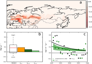
Figure 4. Land abandonment during the WWII and corresponding impact on soil carbon stocks. (a) geographical distribution of cropland reduction between 1940–1942 from LUNEW (in pixel fraction units) and (b) corresponding ELUC estimates in 1940–1949 from TRENDYv4 (S2–S3) and ORCHIDEE-MICT simulations performed here, using LUREF (yellow, SnoLUC – SRef), and the two scenarios corresponding to LUNEW (FOR in dark green, SnoLUC – SFOR and GRA in light green, SnoLUC – SGRA). (c) Post-abandonment changes in soil-C stocks for the two scenarios (FOR and GRA, cropland being followed by forest or grassland establishment, respectively), positive values indicate soil C accumulation. For SGRA, we comparethe changes in soil-C with the values provided by the logistic models in [9] for observed changes in soil carbon observed in Russian territory for grassland expansion in former arable land following abandonment in the 1990s (green dashed line model for all soil types, and shaded area observed range dependent on soil type).
Download figure:
Standard image High-resolution image
Table 2. Comparison of simulated data on C fluxes and stocks with literature values. Values are in Pg C . yr−1 for carbon fluxes (NPP, net sink), and in PgC for C-stocks (soil and biomass C).
| Variable | Region | Period | SRef | SFOR | SGRA | Observation | Ref. |
|---|---|---|---|---|---|---|---|
| Net C sink | Russia, Ukraine, Belarus and Kazakhstan | 1985–2008 | 0.5 | 0.6 | 0.6 | 0.3–1.4 | [8] |
| Russia | early 1990s | 0.8–1 | [9] | ||||
| Russia | 2000–2004 | 0.6–0.7 | [43] | ||||
| NPP | Russia | early 1990s | 4.0 | 4.2 | 4.2 | 4.4–4.5 | [7] |
| Soil C | FSU | 1999a | 846 | 836 | 853 | 709 | [3] |
| Russia and Ukraine agric. | 2000 | 6.8 | 8.4 | 9.7 | 8.8 | [46] | |
| Vegetation C | Russian Forests | 1993 | 46.1 | 45.2 | 45.0 | 43.2 | [44] |
| FSU | 1993–1999 | 44.7 | 49.6 | 44.7 | 43.8 | [45] |
aThe dataset in [3] is calculated from two distinct observation-based datasets for 'present day' period, therefore we compare it with the last year of our simulations.
Several works have shown that cropland abandonment following the collapse of the FSU in the 1990s resulted in increased carbon sequestration due to subsequent natural vegetation growth [38, 39, 40]. Considering the studies summarized by [40], C sequestration in Russian soils during the first 10–15 years following abandonment ranged from 47–129 gC . m−2 . yr−1 (table 3). The climate conditions of the late 20th century were different from the 1940s and cropland area recovered slowly from 1944 onwards attenuating differences in ELUC and C-sequestration from abandonment. Still, SFOR and SGRA estimate increased C-sequestration in abandoned areas of 101 gC . m−2 . yr−1 and 130 gC . m−2 . yr−1 in 1942–1957, consistent with the values in [40]. We compare the post-abandonment trajectories of soil-C for FOR and GRA scenarios with the curves from [9], derived from direct observations of grassland soil-C in arable lands of different soil-types abandoned in the 1990s in Russia (figure 4(c)). The dynamics of SGRA is very close to the mean values in [9], showing that our simulations are able to realistically simulate post-abandonment grassland expansion.
Based on model experiments between 800 and 1850 (AD), [41] suggested that massive land-abandonment due to wars could temporarily enhance the terrestrial sink. Relying on model simulations, [42] proposed that LUC could partly explain the stall in atmospheric CO2 during the 1940s. The two simulations using LUNEW estimate ELUC during the 1940 45% (FOR) to 78% (GRA) lower than the ELUC calculated using LUREF. Our simulations indicate that land-abandonment in FSU during the peak of WWII could increase CO2 uptake by 0.04–0.07 Pg C.yr−1, i.e. 6%–10% of the gap sink between observations and reconstructions of atmospheric CO2 growth rate during the 1940s [2].
3.3. Comparison with observations
To evaluate whether simulated carbon fluxes and stocks are compatible with the observational-record, we compare simulated values with observation-based data for the late 20 C (table 2). Generally, simulated values show good agreement with observation-based data of carbon fluxes and pools in the 1990s and early 2000s (table 2), especially those calculated using LUNEW data. NBP values are within the different observation-based estimates, while NPP is underestimated by 5%–11%. Even if they are forced with the same cropland area, SFOR and SGRA differ in their estimates of soil-C in crops by 1.3 PgC over Russia and Ukraine in 2000, highlighting the relevance of slow processes and legacy effects from LUC on C-stocks. Simulated forest C in Russia in 1993 is 4%–7% higher than the values reported by [44]. Total vegetation C stocks simulated by SRef and SGRA between 1993 and 1999 are very close to those reported by [45], and overestimated by 13% by SFOR. Soil carbon in cropland areas simulated by SFOR is very close to the literature values [46].
4. Conclusions
Here, we simulate CO2 fluxes in northern Eurasia using a model specifically developed for high-latitudes, in order to evaluate two hypothesis to explain the differences between observations and reconstructions of the GCB in the early 20th century [2].
The high-latitude warming during the 1930s and 1940s is a consistent feature in observation-based and proxy data [13, 17, 47]. Our simulations indicate very strong enhancement of net CO2 uptake in northern Eurasia by 0.4 PgC.yr−1, vegetation growth and accumulation of carbon in soils in the high-latitudes coinciding with spring warming, which is supported by tree-ring data [4]. The fact that state-of-the-art LSMs from TRENDYv4 do not capture such response highlights the importance of correctly representing and parametrizing high-latitude processes to capture the effects of warming on boreal vegetation. The climate-induced enhancement of NBP in northern Eurasia could potentially explain 60% of the 1940s' global sink gap found in [2].
Table 3. Carbon sequestration in former arable soils following the collapse of the FSU in the 1990s (adapted from the values provided by the review from [40]), and following the cropland abandonment between 1940–1942. Since most of the reference values cover a period of ca. 15 years, we present the results for a period of 15 years following massive cropland decrease: 1942–1957.
| Period | Average C-sequestration (gC . m−2 . yr−1) | Method | Study |
|---|---|---|---|
| 1990–2004 | 129 | Approximation | [49] |
| 1990–2005 | 55 | RothC-model | [50] |
| 1990–2006 | 114–126 | Soil-GIS, approximation | [9] |
| 1991–2000 | 47 | ORCHIDEE model | [38] |
| 1990–2001 | 92–96 | Soil-GIS, approximation | [40] |
| 1942–1957 | 101 | ORCHIDEE-MICT | SFOR |
| 1942–1957 | 130 | ORCHIDEE-MICT | SGRA |
Massive and abrupt land-abandonment in the 1920s and 1940s in the FSU and subsequent recovery of C-stocks could result in increased terrestrial uptake. Such short-term fluctuations are not represented in the LUC datasets used to force LSMs, as their main purpose is to estimate ELUC over centuries [26]. We compiled a new dataset of cropland area in the FSU based on annual official stastistics from GOSKOMSTAT collected between 1913 until 1961. Our dataset is consistent with other social and economical statistics, indicating that the changes in cropland area reported in our dataset are realistic. Here we show that extreme but relatively short LUC events may result in decadal ELUC variability and contribute to the discrepancies found in [2]. Focusing on the massive cropland area decrease during 1940–1942, we find a reduction of ELUC in the 1940s of 0.04–0.07 PgC.yr−1 using LUNEW, compared to LUREF. The reduction in ELUC due to land-abandonment reported by LUNEW corresponds only to a small fraction of the 1940s global sink gap in [2] (6%–10%), so more research is needed to attribute this gap to anthropogenic and natural carbon cycle processes. However, land-abandonment during WWII not reported in HYDE3.1 likely occurred in other regions, e.g. China [48]. Additionally, other processes may further contribute to an increased sink in the 1940s, e.g. nutrient deposition from fossil fuel burning, or changes in agricultural practices, fertilizer use and wood harvest.
Besides providing an estimate of the potential contribution of LUC and climate variability to uncertainty in the GCB, our study highlights two important aspects for the carbon-cycle community. On the one hand, we show the importance of representing specific high-latitude processes to better simulate the terrestrial sink response to arctic warming. On the other hand, we show the relevance of using LUC datasets with finer temporal resolution during periods of drastic demographic and economic transitions, to estimate resulting LUC emissions and their variability. Still, our results point to key processes that may need to be improved in land-surface models and LUC datasets in order to better represent decadal variability in the land CO2 sink.
5. Data availability
The full dataset including the regional values when available, and detailed information about the data sources are provided in supplementary material.
Acknowledgments
The work is supported by the Commissariat à l'énergie atomique et aux énergies alternatives (CEA). The authors would like to thank the TRENDY modelling teams and S Sitch and P Friedlingstein for providing and maintaining the TRENDYv4 outputs. Above-ground biomass C stocks from [45] were downloaded from www.wenfo.org/wald/global-biomass/. We thank the valuable help of Dan Zhu, Fabienne Maignan, Shushi Peng & Albert Jornet during the development of this study.