

Abstract
Recent studies have assessed the impacts of climate change at specific global temperature targets using relatively short (30 year ) transient time-slice periods which are characterized by a steady increase in global mean temperature with time. The Inter-Sectoral Impacts Model Intercomparison Project Phase 2b (ISIMIP2b) provides trend-preserving bias-corrected climate model datasets over six centuries for four global climate models (GCMs) which therefore can be used to evaluate the potential effects of using time-slice periods from stabilized climate state rather than time-slice periods from transient climate state on climate change impacts.
Using the H08 global hydrological model, the impacts of climate change, quantified as the deviation from the pre-industrial era, and the signal-to-noise (SN) ratios were computed for five hydrological variables, namely evapotranspiration (EVA), precipitation (PCP), snow water equivalent (SNW), surface temperature (TAR), and total discharge (TOQ) over 20 regions comprising the global land area.
A significant difference in EVA for the transient and stabilized climate states was systematically detected for all four GCMs. In addition, three out of the four GCMs indicated that significant differences in PCP, TAR, and TOQ for the transient and stabilized climate states could also be detected over a small fraction of the globe. For most regions, the impacts of climate change toward EVA, PCP, and TOQ are indicated to be underestimated using the transient climate state simulations. The transient climate state was also identified to underestimate the SN ratios compared to the stabilized climate state. For both the global and regional scales, however, there was no indication that surface areas associated with the different classes of SN ratios changed depending on the two climate states (t-test, p > 0.01).
Transient time slices may be considered a good approximation of the stabilized climate state, for large-scale hydrological studies and many regions and variables, as: (1) impacts of climate change were only significantly different from those of the stabilized climate state for a small fraction of the globe, and (2) these differences were not indicated to alter the robustness of the impacts of climate change.
Export citation and abstract BibTeX RIS

Original content from this work may be used under the terms of the Creative Commons Attribution 3.0 licence.
Any further distribution of this work must maintain attribution to the author(s) and the title of the work, journal citation and DOI.
1. Introduction
Identifying an optimal long-term target for global warming is difficult due to diverse goals and priorities valued by countries (Hallegatte et al 2016). Nevertheless, by signing the Paris agreement, almost all countries have agreed to adopt a global temperature target well below 2.0 °C above the pre-industrial global mean temperature and pursue efforts to limit the temperature increase to 1.5 °C above pre-industrial levels (UNFCCC 2015). Following the ratification of the Paris agreement, the Intergovernmental Panel on Climate Change (IPCC) was requested to produce a special report in 2018, highlighting the impacts of global warming of 1.5 °C above pre-industrial levels (Hallegatte et al 2016, Schellnhuber et al 2016).
The impacts of climate change under various emission scenarios using stabilized greenhouse gas concentrations in the atmosphere were evaluated previously (Gao et al 2017), and recent studies have started to assess the impact of climate change at specific global temperature targets (Arnell et al 2016, Donnelly et al 2017). The analyses were performed using time-slice periods (typically 30 years long). These time-slice periods are centered around the year when the global mean temperature (GMT) reaches a global temperature target. Relevant variables for the study are then extracted for the given period. This technique assumes that the effect of time-lag in the relevant systems are of minor importance for the indices studied (Schleussner et al 2016). In addition, these time-slice periods are transient (transient climate state), characterized by a steady increase in GMT with time (Knutti et al 2016, Donnelly et al 2017). While it would be preferable to conduct such climate change impact analyses under the condition that the GMT is stabilized at the examined global temperature targets (stabilized climate state), such targeted simulations are however not available for most combinations of climate models and global temperature targets, including the global warming of 1.5 °C above pre-industrial levels (figure S0). Consequently, studies that have evaluated climate change impacts at specific global temperature targets so far have relied on transient climate states which may, however, misrepresent the real impacts of global warming in a stabilized climate state of the same temperature.
The Inter-Sectoral Impact Model Intercomparison Project (ISIMIP) was created to incorporate multiple hydrological models (as well as other impact models), global circulation models (GCMs), representative concentration pathways (RCPs), and shared socio-economic pathways (SSPs) in climate change studies (Warszawski et al 2014). The recent ISIMIP2b protocol was designed to support the IPCC Special Report on the 1.5 °C target (Frieler et al 2016) and is particularly suited for evaluating the potential impacts of using indicators from a stabilized climate state rather than indicators from a transient climate state. ISIMIP2b provides bias-corrected climate model datasets spanning long time periods that incorporate both transient and stabilized climate states (figure S0).
This study aims to quantify the impacts of the transient and stabilized climate states of equivalent GMT on hydrological variables over the globe. Specific objectives, defined over the globe and regions, are to: (1) identify whether a quantifiable difference between the hydrological impacts for transient and stabilized climate states can be detected, (2) determine if the robustness of the hydrological impacts is influenced by the choice of climate state.
2. Materials and methods
2.1. Input datasets and hydrological model
We used datasets from four global circulation models (GFDL-ESM2M, MIROC5, IPSL-CM5A-LR, and HadGEM2-ES), bias corrected following Hempel et al (2013) and Lange (2017) in conjunction with an established global hydrological model, the H08 model (Hanasaki et al 2017), to generate variables, relevant for the water cycle: mean monthly (1) precipitation (PCP), (2) snow water equivalent (SNW), (3) evapotranspiration (EVA), (4) surface temperature (TAR), and (5) total discharge (TOQ). The four eras defined by the ISIMIP2b protocol are: pre-industrial (1660–2299), historical (1860–2005), future (2006–2099), and future-extended (2100–2299). The rationales behind the choice of the RPCs, eras, and more modeling choices included into the ISIMIP2b protocol can be found in Frieler et al (2016).
The H08 model is a global hydrological model that operates daily at a 0.5° × 0.5° spatial resolution with water and energy balance closure. Both natural and anthropogenic water flow are simulated by the model. H08 is open-source and source code and manuals can be accessed online (http://h08.nies.go.jp). In this study, an enhanced version of H08 was used (Hanasaki et al 2017). Additional information regarding the processes implemented in H08 can be accessed via the underlying H08 references (Hanasaki et al 2008a, 2008b, Hanasaki et al 2010).
We first analyzed when specific temperature thresholds above pre-industrial levels were achieved using multiple moving GMT averages (Vautard et al 2014). Here, pre-industrial levels correspond to the entire pre-industrial simulation (nominally spanning the years 1661–2299) of the respective GCMs. To evaluate the impact of climate change on the variables, 30 year periods were extracted, centered on the year in which global warming thresholds were reached (figure S0). To objectively compare the variables for the transient and stabilized climate states, the same GMT threshold was used for both states. The GCMs used in this study stabilized around +1.7 °C (GFDL-ESM2M, and MIROC5), +2.6 °C (IPSL-CM5A-LR), and +1.9 °C (HadGEM2 E S) relative to the pre-industrial era. A 30 year period of data, analogous to the transient dataset, was extracted within the stabilized period, for each GCMs, the 30 year average surface temperature is identical between the transient and stabilized climate states. The resulting stabilized datasets used in this study consisted of 2069–2099 for GFDL-ESM2M, 2170–2200, for MIROC5, 2184–2214 for IPSL-CM5A-LR, and 2185–2215 for HadGEM2 E S, respectively (figure S0). The periods used for the transient climate state were in contrast within the 21st century: 2014–2044, 2016–2046, 2017–2047, and 2016–2046 for GFDL-ESM2M, MIROC5, IPSL-CM5A-LR, and HadGEM2 E S, respectively. The whole range of the transient period is hence referred as the first half of the 21st century in text. The whole range of the stabilized period of three GCMs, excluding GFLD-ESM2M, is 2170–2215 and hence referred as the late 22nd century in text. The outputs of GFLD-ESM2M was excluded from the stabilized period since it is very different from others. This does not influence our findings, as indicated in all supplementary figures available at stacks.iop.org/ERL/13/064017/mmedia which include the stabilized period for GFLD-ESM2M.
The sources of uncertainty associated with the years when the GMT reaches specific levels of global warming were separated using the methodology described by Hawkins and Sutton (2011). Briefly, internal variability is estimated using a fourth-order polynomial fit, model uncertainty is assessed by analyzing model spread around the mean for each given scenario and the scenario uncertainty is given by the deviation between the multi-model means for each scenario (Hawkins and Sutton 2011). Averaging across multiple global warming thresholds (+1.5 °C to +3 °C), the years when the GMT reached global temperature thresholds varied by ±2.79 and ±2.89 years, due to natural variably and GCMs, respectively. Considering the control periods, GCMs ensemble, and window size of moving average used to estimate when specific global warmings are achieved, these results are in line with the literature (table S1).
2.2. Impacts of climate change and quantification of robustness
The impacts of climate change in a transient and stabilized climate states were analyzed for an equally warmer world relative to pre-industrial levels, using 30 year of data. The impacts of climate change were quantified as the relative deviation from the pre-industrial era and were computed on the 0.5 by 0.5 grid for all variables obtained for the transient and stabilized climate states:
where future is the mean value of the variable for the future scenario (transient or stabilized climate states), and picontrol is the mean value of the variable for the pre-industrial period. The hydrological impacts at the grid box and regional scales were investigated using 21 land regions (Giorgi and Francisco 2000) defined in table S2, which were designed to give a broader picture of the potential hydrological impacts of climate change than a selection of river basins (Davie et al 2013). The significance of the shift in impacts due to climate change for the transient and stabilized climate states was further assessed at individual grid boxes, relative to model-based estimates of natural variability (Karoly and Wu 2005). Briefly, the differences in variables between the transient and the stabilized were first calculated. Then, a t-test was used to assess the fraction of area where these differences were significantly different from zero. Using a Monte Carlo (MC) procedure, the differences in non-overlapping 30 year periods of the pre-industrial era were computed 1000 times and, we evaluated at each grid point the significance of the difference at the 95% level. Last, using the MC outputs, the 5th–95th percentile range of the fraction of area detected as significantly different due to natural variability was calculated (Karoly and Wu 2005).
Various methods to synthesize the different projections in a multi-model approach and to assess the robustness of predictions were developed (Knutti and Sedlacek 2013). Among the methods available, the signal-to-noise (SN) ratio and the sign consensus methods were reported to generate similar conclusions (Power et al 2012). Due to the relative low number of GCMs available in this study, the SN ratio method was selected to indicate areas of the globe experiencing robust hydrological alterations due to climate change using both the transient and stabilized climate runs. The SN ratios defined by the IPCC Third Assessment Report (IPCC 2013), were calculated individually for each grid cell, and for the entire sequence of monthly values within a given 30 year period:
where SN is the signal to noise ratio of a specific variable, Δ is the difference between the mean value of a variable for the experimental and control periods, and σ is the standard deviation over the control period of the variable (Hawkins and Sutton 2011). The SN ratio represents the strength of the change signal compared to natural variability (noise), and the signal stands out against the noise when and where this ratio is large (IPCC 2013).
3. Results and discussion
3.1. Hydrological impacts for the transient and stabilized states
Globally, the differences in the forecasted impacts of climate change between the transient and stabilized climate state were difficult to observe as the transient climate state did not systematically result in under- or over-estimates of the impacts of climate change compared to those predicted using the stabilized climate state (figure S2). The mean and the 95th percentile differences in impacts between the transient and stabilized climate states were calculated for all latitude bands and all variables (figure S3). Spikes in the differences between impacts forecasted at the transient and stabilized climate states were located mainly at low latitude for EVA and PCP, medium latitude for SNW, and low and high latitudes for TOQ, respectively. While these spikes are often associated with wide uncertainty bands, in such regions and for the above-mentioned variables, relying on the transient climate state dataset misrepresents the real impacts of global warming. Figure S3 also highlighted the great uncertainty encompassed in predicting the impacts of SNW as the sign and magnitude of the impacts differed greatly for all GCMs.
Table 1 presents the fraction of surface area (%) where significant differences in hydrological variables between the transient and the stabilized climate states were detected (t-test p < 0.05) for all GCMs (including GFDL-ESM2M). These numbers however need to be compared with the range of surface area (5th and 95th percentiles) where significant differences between 30 year periods of the pre-industrial era arise from natural variability. While the percentage of land surface projected to experience significant difference between the transient and stabilized climate states varied, MIROC5, IPSL-CM5A-LR, and HadGEM2-ES indicated that those were higher than what is expected from natural variability for PCP, EVA, TAR, and TOQ. Overall, the GCMs therefore indicate minor but significant differences in PCP, EVA, TAR, and TOQ between the transient and stabilized states. In contrast, GFDL-ESM2M only highlighted EVA as significantly different between the transient and stabilized states (table 1). While the 30 year average global temperature of HadGEM2 E S not the warmest (+1.9 °C), it was generally associated with large differences on climate change impacts between transient and stabilize climate states (table 1). In contrast, the 30 year average global temperature of GFDL-ESM2M was the lowest (+ 1.7 °C) and it related to the smallest differences in climate change impacts of all GCMs (table 1). In addition, as previously indicated, the stabilized period used for GFDL-ESM2M is very different from that of the other GCMs and is relatively close to the transient period which may explain the non-significant differences observed for this GCM only.
The average impacts of climate change (over four GCMs) on the five variables over 21 regions and the globe for the transient and stabilized climate states are illustrated in figure 1. The difference in trends between the impacts simulated for the transient and stabilized climate states vary greatly, depending on the combination of regions and hydrological variables. Additionally, for few combinations of regions and variables, the differences in impacts between the transient and stabilized climate states were extremely vulnerable to outliers, this is highlighted with the low r2 in figure 1. Overall, the slopes of the linear regressions applied in figure 1 were highly significant (ANOVA, p < 0.01) for all variables and higher than 1 for EVA, PCP, and TOQ. In contrast, the slopes of the regression equations obtained for TAR and SNW were significantly lower than 1 even if the outlier data for South Africa was removed from the latter variable dataset. Accordingly, for most Giorgi regions, the impacts of climate change for EVA, PCP, and TOQ are indicated to be underestimated using the transient climate state simulations. For TAR and SNW (figure 1), since the slope of the regression line is smaller than that of the 1:1 line fitted for all regions, the impacts of climate change on the two variables for the transient climate state were underestimated in the right of figure 1, but in contrast, overestimated in the left of figure 1 (e.g. impact of SNW for SSA region). The impacts of climate change were most critically underestimated using the transient climate state simulations in: East Asia (EAS), South Asia (SAS), and northern Europe (NEU) for evapotranspiration; East Asia (EAS), and Tibet (TIB) for precipitation; North Asia (NAS), Australia (AUS), Central America (CAS), and southern South America (SSA) for total discharge, respectively (figure 1). In some Giorgi regions, the presence of outliers compromised the accurate representation of the impacts of climate change for the two climate states (e.g. Greenland and South Africa for precipitation, and snow water equivalent, respectively). In general, those were associated with major uncertainty indicating that the different GCMs did not necessarily agree on the sign or magnitude of the impacts. The Giorgi regions consist of aggregated areas exhibiting very contrasted snow and discharge regimes (e.g. Australia, Central America). This may have contributed to some of the extreme uncertainty displayed in figure 1. In addition, overall, temperature increases over the globe, but trends in precipitation and snow fall are diverse (Krysanova and Hattermann 2017), increasing the variety of trends over the Giorgi regions.
Quantifiable, significant but generally small differences between the estimated hydrological impacts for the transient and stabilized climate states were detected over the globe and at the regional scale. It remains to determine whether these differences in hydrological impacts are affecting the detection of areas of the globe flagged as experiencing robust change in hydrological variables due to global warming.
3.2. Robustness of hydrological impacts for the transient and stabilized climate states
Table 1. Fraction of surface area (%) over the globe with differences between the transient and the stabilized locally significant at the 95% level. The number in brackets is the result of a field significance test to determine the value of this fraction due to natural variability (5th and 95th percentiles). Variables for which the differences between the transient and stabilized climate states are higher than what can be expected due to natural variability are highlighted in grey.
| Variables | GCMs | |||
|---|---|---|---|---|
| GFDL-ESM2M | MIROC5 | IPSL-CM5A-LR | HadGEM2 E S | |
| PCP | 0.34% (0.01%–0.62%) | 1.21% (0.06%–0.61%) | 1.19% (0.15%–1.07%) | 2.73% (0.07%–0.98%) |
| SNW | 0.99% (0.90%–1.11%) | 0.85% (0.90%–1.10%) | 0.79% (0.91%–1.21%) | 1.11% (0.92%–1.02%) |
| EVA | 0.87% (0.09%–0.79%) | 7.13% (0.10%–0.57%) | 1.56% (0.14%–1.23%) | 4.61% (0.10%–0.78%) |
| TAR | 1.33% (0.07%–1.58%) | 3.76% (0.06%–3.15%) | 3.56% (0.49%–2.94%) | 4.63% (0.58%–3.46%) |
| TOQ | 4.48% (2.32%–4.96%) | 5.80% (3.44%–5.11%) | 5.87% (2.74%–4.24%) | 7.40% (2.71%–4.26%) |
The average SN ratios of the Giorgi regions were calculated for the transient and stabilized climate states (figure 2). The slopes of the linear regressions applied in figure 2 were all significantly higher than 1 (ANOVA, p < 0.01) for all variables. Consequently, the transient climate state tends to underestimate the SN ratios of the stabilized climate state. In addition, the regions in which the SN ratios of the stabilized climate state were the most underestimated using the transient climate were consistent with the previous analysis of impacts of climate change.

Figure 1. Average hydrological impacts (over four GCMs) for the transient and stabilized climate states over Giorgi regions. The grey area represents the uncertainty encompassed in the regions and extends one standard deviation from the mean. The black line is the identity line and the green line is a linear regression across all regions.
Download figure:
Standard image High-resolution image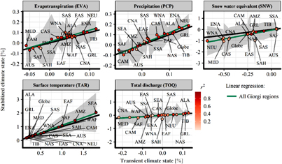
Figure 2. Average SN ratios (over four GCMs) for the transient and stabilized climate states over the Giorgi regions. The grey area represents the uncertainty encompassed in the regions and extends one standard deviation from the mean. The black line is the identity line and the green line is a linear regression across all regions.
Download figure:
Standard image High-resolution imageThe robustness of the predicted hydrological impacts was quantified by computing SN ratios equation (2) for the transient and stabilized climate states. Compared with the literature (see the following references), the resulting SN ratios were relatively low which can be attributed to the different aggregation methods used to evaluate SN ratios. Higher SN ratios can be expected when using: (1) averaging indicators over the globe or specific regions (Karmalkar and Bradley 2017), (2) separately computing the SN ratios for different seasons (Giorgi and Francisco 2000), (3) using 10 to 30 year averages indicators in the calculation (Giorgi and Bi 2009), and (4) relying on model ensemble rather than a pre-industrial period to compute the standard deviation of the variables (Donnelly et al 2017).
To evaluate if the increase in SN ratios for the stabilized climate state impacted the identifications of areas flagged as experiencing robust change in hydrological variables due to climate change, the SN ratios for the transient and stabilized states were re-classified into five groups: negligible (SN ≤ 0.20), low (0.20 < SN ≤ 0.4), medium (0.4 < SN ≤ 0.6), high (0.6 < SN ≤ 1), and very high (SN>1). The thresholds used to define the different groups are rather arbitrary but Power et al (2012) demonstrated that: (1) for SN ratios lower than 0.2 there is almost no consensus among the predictions of the models, (2) for SN ratios higher than 0.2 but lower than 0.4 there is a consensus among model forecasts indicating that change is unremarkable, and (3) for SN ratios higher than 0.4, there is a high level of consensus among the models indicating a remarkable change. For all Giorgi regions, the total surface areas (km2) occupied by the different SN classes was computed for both transient and stabilized climate states (figure S4). Globally, there was no indication that the surface areas associated with the different classes of SN ratios changed depending on the two climate states (t test, p > 0.01). At the regional scale, some minor differences were observed in surface areas experiencing robust change in various variables (figure S4) but none were significant (t test, p > 0.01).
4. Summary and discussions
Hydrological variables obtained for the transient and stabilized climate states and corresponding to equally warmer worlds were significantly different over small portions of the globe, and when looking at specific Giorgi regions for most GCMs. Regions where the impact of climate change were significantly underestimated using the transient climate state were East Asia, South Asia, and northern Europe for evapotranspiration, East Asia, and Tibet for precipitation, North Asia, Australia, Central America, and southern South America for total discharge, respectively. In particular, the precipitation response to global warming appears to be slightly 'wetter' (more increase, or less decrease in precipitation) for the stabilized state than for the transient state in regions like western North America, East Africa, the Middle East, southern Siberia, and southern China (figure S6).

Figure 3. Annual average (a) increase in global land surface temperature relative to pre-industrial level (b) concentration in CO2. Note: the coloured bands in (a) indicate ±1 standard deviation of the GCMs ensemble.
Download figure:
Standard image High-resolution image
Previous studies have discussed the possible mechanisms of different changes in hydrological cycle between the transient and stabilization stages. Generally, the concentrations of CO2 and other greenhouse gases (GHGs) are higher during the first half of the 21st century than during the late 22nd century as indicated in figure 3(b) and table S3. Higher concentrations of CO2 for an identical GMT changes would lead to weaker precipitation (and evaporation) responses due to greater atmospheric adjustments such as: cloud development, cloud cover, cloud properties, atmospheric stratification, and energetic re-equilibration of the atmosphere (Sherwood et al 2015, Allen and Ingram 2002, Dinh and Fueglistaler 2017, Kamae et al 2015).
The changes in global mean precipitation could also be partly driven by different emissions of aerosols (Pendergrass and Hartmann 2012, Shiogama et al 2010b, Shiogama et al 2010a). Indeed, the emissions of various air pollutants change significantly over time, in the RCP2.6 scenario (Lamarque et al 2011, Meinshausen et al 2011). In general, these emissions (except those of ammonia) decrease around the first half of the 21st century while remaining nearly constant during late 22nd century, as indicated in table S4. Reduction in emissions are mostly achieved over time due to an overall decrease in coal use. In contrast, the emission of some pollutants (e.g. NH3) increase due to shift in the agricultural sector toward biofuel production. The precipitation sensitivity per a 1 °C GMT warming is higher for aerosols (especially black carbon aerosols) than that for the well mixed greenhouse gases (Pendergrass and Hartmann 2012, Shiogama et al 2010b, Shiogama et al 2010a). This therefore does not explain the slightly higher precipitation sensitivity in the stabilized climate state than in the transient climate state that we find in few regions (figure S6).
As a third possible mechanism, land-ocean warming contrasts are a fundamental response of the climate system to global warming and were reported to persist in an equilibrium climate state (Byrne and O'Gorman 2013). Land-ocean warming contrasts primary arise due to differences in lapse rates over land and ocean due to the limited moisture available over land (Byrne and O'Gorman 2013). Some differences in soil moisture levels between the transient and stabilization stages may be driven by change in stomatal conductance and evapotranspiration in elevated CO2 environments and would indirectly modify the land-ocean warming contrast during the two climate states. In general, a reduction in relative humidity over land while maintaining a relatively constant humidity and temperature over oceans was reported to increase further temperature over land (Byrne and O'Gorman 2013). This imply that land-ocean warming contrasts are potentially higher during the first half of the 21st century which experiences elevated greenhouse gas concentrations as compared to those of the late 22nd century. Changes in the land-ocean warming contrasts would further affect the moisture transport between the land and the ocean and the spatial distribution of precipitation responses (Mitchell et al 2000). The mechanisms of different changes in hydrological cycle between the transient and stabilization stages are however beyond the scope of this work, and we remain testing these hypotheses for a future work.
The transient climate state was identified to underestimate the SN ratios of the stabilized climate state. But for both the global and region scales, there were no indication that surface areas associated with the different classes of SN ratios changed depending on the two climate states (t test, p > 0.01). In conclusion, transient time slices may be considered a good approximation of the stabilized state for large-scale hydrological studies and many regions and variables, but may be less ideal when analyzing the above-mentioned regions and variables. In addition, since this study focused on RCP2.6 and relatively low increase in GMT relative to pre-industrial levels (maximum increase of +2.6 °C for IPSL-CM5A-LR), these results between transient and stabilized may not hold for higher increase in GMT (e.g. RCP6.0, RCP8.5), due to potential environmental tipping points. These findings should be considered when assessing the impacts of global warming levels at other levels of global warming, consistent with the Paris Agreement.
Acknowledgments
This research was supported by MEXT/JSPS KAKENHI; Grant number: 16H06291. H S was supported by the Integrated Research Program for Advancing Climate Models (TOUGOU program) from the Ministry of Education, Culture, Sports, Science and Technology, Japan and ERTDF 2–1702 of Environmental Restoration and Conservation Agency, Japan. J S received funding from the BMBF in the framework of ISIMIP2b, grant number 01LS1201A2. We thank the CMIP modelling groups for making available their model output.