

Abstract
The assessment of health impacts associated with airborne particulate matter smaller than 2.5 μm in diameter (PM2.5) relies on aerosol concentrations derived either from monitoring networks, satellite observations, numerical models, or a combination thereof. When global chemistry-transport models are used for estimating PM2.5, their relatively coarse resolution has been implied to lead to underestimation of health impacts in densely populated and industrialized areas. In this study the role of spatial resolution and of vertical layering of a regional air quality model, used to compute PM2.5 impacts on public health and mortality, is investigated. We utilize grid spacings of 100 km and 20 km to calculate annual mean PM2.5 concentrations over Europe, which are in turn applied to the estimation of premature mortality by cardiovascular and respiratory diseases. Using model results at a 100 km grid resolution yields about 535 000 annual premature deaths over the extended European domain (242 000 within the EU-28), while numbers approximately 2.4% higher are derived by using the 20 km resolution. Using the surface (i.e. lowest) layer of the model for PM2.5 yields about 0.6% higher mortality rates compared with PM2.5 averaged over the first 200 m above ground. Further, the calculation of relative risks (RR) from PM2.5, using 0.1 μg m−3 size resolution bins compared to the commonly used 1 μg m−3, is associated with ±0.8% uncertainty in estimated deaths. We conclude that model uncertainties contribute a small part of the overall uncertainty expressed by the 95% confidence intervals, which are of the order of ±30%, mostly related to the RR calculations based on epidemiological data.

Original content from this work may be used under the terms of the Creative Commons Attribution 3.0 licence.
Any further distribution of this work must maintain attribution to the author(s) and the title of the work, journal citation and DOI.
1. Introduction
Exposure to airborne fine particulate matter (diameter less than 2.5 μm, or PM2.5) has been associated with a number of short- and long-term adverse health outcomes varying from respiratory illnesses to premature death (Dockery et al 1993, 2009, Pope et al 2002, 2004, 2009, Filleul et al 2005, Krewski et al 2009, Ostro et al 2010, Rückerl et al 2011, Beelen et al 2014). The assessment of health impacts from ambient (outdoor) air pollution relies on an integrated methodology that uses observations and/or air quality models to determine pollutant concentration distributions, and synthesizes this information with exposure and population vulnerability on national and global scales (Cohen et al 2005, Anenberg et al 2010, Li et al 2010, Pozzer et al 2012, Fann et al 2012, Lelieveld et al 2015, Giannadaki et al 2017, Pozzer et al 2017). The use of atmospheric modelling systems is necessary, in order to provide information on the PM2.5 concentrations in regions where air quality is not monitored, and to investigate alternative scenarios related to factors such as emissions, air quality regulations and population development.
PM2.5 concentrations are often derived from global models utilizing a grid spacing ranging from 100 km–400 km (Bey et al 2001, West et al 2006, Anenberg et al 2010, 2012). Many of the species that comprise a PM2.5 total mass concentration are formed in the atmosphere from chemical reactions between precursor species (Thompson et al 2014). Strong spatial concentration gradients of emissions can influence chemical production, and may lead to errors at too coarse a resolution due to spatial averaging of emissions (Thompson et al 2014). Thus, the use of coarse grid resolutions, necessitated by computational resource limitations and global model parameterisations, may result in the underestimation of peak concentrations in densely populated and industrialized areas (Punger and West 2013, Li et al 2010). This could influence mortality estimates by misrepresenting the gradients between pollution and population distributions, leading to errors in estimates of health impacts. Grid resolution is expected to affect differently the primary and secondary aerosols; therefore, an analysis of PM components instead of total particulates might be interesting (US EPA 2007, Punger and West 2013), warranting further investigation of spatial resolution to different airborne aerosol species. For applications on urban and regional scales, several studies have investigated how estimates of health impacts at coarser resolutions differ from those at fine resolutions (Punger and West 2013, Thompson et al 2014) with contradictory results. Punger and West (2013) reported that coarse grid resolutions produce national mortality estimates in the USA that are substantially low-biased. However, Thompson et al (2014) did not find a significant response of health impacts associated with changes in PM2.5 concentrations to model resolution. A robust conclusion is pending.
In this study, we performed several sensitivity tests to identify the uncertainty range introduced to the mortality calculations related to the grid spacing of the modelling system, the vertical distribution of the PM2.5 concentrations, and the bin size of the relative risk factor concentration step. We also calculated mortality rates from aerosol concentrations derived from satellite retrievals of the aerosol optical depth (AOD) for the same year (2014), from various satellite instruments (NASA MODIS, MISR, and SeaWIFS), as discussed in van Donkelaar et al (2016). Here we assess the relative differences between simulations and observational analysis relative to the 95% confidence interval in the estimation of the rates of mortality and disease, as derived from the epidemiological studies on the relative risk of disease.
This paper is organised as follows: section 2 gives a brief description of the methodology and tools used in this work. In section 3 the results of the uncertainties driven by the options used in the calculation of the mortality estimates are presented and discussed, while section 4 summarises the main findings of this work and proposes focus points for future analysis.
2. Methodology
We used the Weather Research and Forecast model coupled with Chemistry (WRF-Chem) version 3.6.1 to simulate particulate matter over Europe for the year 2014 (Grell et al 2005, Fast et al 2006). This modelling system includes meteorological and chemical modules that are fully consistent, as they apply the same transport scheme (mass and scalar preserving), physical schemes for subgrid-scale transport, and the same spatial and temporal configuration. WRF-Chem was configured over Europe and uses two domains, one with a horizontal resolution of 100 km and the other of 20 km, nested into the coarse grid domain. For both simulations, the following physical and chemical options are used. The second generation Regional Acid Deposition Model mechanism (Stockwell et al 1990) is applied to simulate the gas phase chemistry. The aerosol modules used are the Modal Aerosol Dynamics Model for Europe (Ackermann et al 1998) for inorganic species, and the Secondary Organic Aerosol Model (Schell et al 2001) for secondary organic aerosols. The aerosol size distribution is described with three log-normal modes (Αitken, accumulation, and coarse). The options for the physical parameterisations are the following: the Morrison microphysics scheme (Morrison et al 2005), the MM5 similarity surface layer scheme (Zhang and Anthes 1982), the Noah Land Surface Model (Chen and Dudhia 2001), the Yonsei University Planetary Boundary Layer scheme (Hong et al 2006), the Grell 3D Ensemble Scheme for cumulus parameterisation (Grell and Dévényi 2002), and the Rapid Radiative Transfer Model radiation scheme (Iacono et al 2008) for both shortwave and longwave radiation budgets.
The initial and boundary conditions for the meteorological data were provided by the National Center for Environmental Prediction global forecast system at a resolution of 0.5° × 0.5°. Land use and soil category data sets from the US Geological Survey (USGS) are used. The initial and boundary conditions for the chemical species are provided from global simulations with the Model for Ozone And Related chemical Tracers version 4 (MOZART-4) model (Emmons et al 2010). Emissions are calculated from the global emission dataset EDGAR-HTAP v2 (Janssens-Maenhout et al 2012). The EDGAR-HTAP dataset has a resolution of 0.1° × 0.1° and provides annual anthropogenic emissions of NOx, SOx, non-methane volatile organic compounds (NMVOCs), CO, NH3, PM2.5 and PM10 covering 11 source sectors (SNAP categories), plus emissions from ships and volcanoes (SOx) for the reference year 2010. In the EDGAR-HTAP v2 dataset, the NMVOCs are lumped into reactive compound categories, and the speciation into groups is based on the approach of Middleton et al (1990). Biogenic emissions (isoprene, monoterpenes and nitrogen emissions by soil) have been calculated on-line from the Model on Emissions of Gases and Aerosols from Nature, using the USGS land-use classification and branch-level emission factors which incorporate canopy shading.
The PM2.5 concentrations derived from the two simulations are compared to measurements reported by European countries to the European Environment Agency (EEA) for 2014 and available in Airbase v. 8 (EEA 2016). The analysis covers all the regulated pollutants in the Air Quality Directives (EU 2004 and EU 2008) in the EU-28 and the European Economic Area member countries whose territories are fully included in the model domains. We use only those monitoring stations with at least 75% of data coverage (the fraction of the year for which valid concentration data is available) for the analysis of fine particles with diameters of 2.5 μm or less. Simulated mass concentrations of total PM2.5 from anthropogenic sources (no mineral dust or sea salt) are then used to derive mortality estimates for several health conditions and age groups.
The diseases taken into account in this study include ischemic heart disease, cerebrovascular disease from ischaemic and haemorrhagic stroke, chronic obstructive pulmonary disease, lung cancer, and acute lower respiratory infections which also affect children. The methodology for the calculation of the mortality and incidence rates of the aforementioned diseases requires the input of spatially resolved PM2.5 concentrations; these values are provided from the simulations of the WRF-Chem modelling system at 100 km and 20 km grid spacing covering the same region (Europe). The mass concentrations are given as annual means per grid cell (100 × 100 km and 20 × 20 km). No observational assimilation or calibration has been performed with ground-level PM2.5 measurements or satellite retrievals, in order to assess the stand-alone predictability of the modelling system and its capability to be used in future emission scenarios.
Other data sets used as input for the calculations (country-level baseline mortality rates for the diseases and population data) have been taken from the WHO Global Health Observatory (www.who.int/gho/database/en/), being representative of the year 2010.
Concentration–response (C-R) functions: we use the methodology of Burnett et al (2014) that builds on the studies of Pope et al (2009, 2011) to constrain the shape of the C-R relationship by developing integrated exposure–response functions (IERs) using a wide range of mortality data capturing a vast range of air quality conditions. These IERs are employed to estimate relative risks attributable to ambient PM2.5 for ischemic heart disease (IHD), cerebrovascular disease and related mortality from ischaemic and haemorrhagic stroke (CEVI and CEVH, respectively), chronic obstructive pulmonary disease (COPD), lung cancer (LC) and acute lower respiratory infection (ALRI). The RR is parameterised in the IER framework following the formulation:
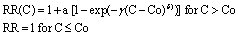
The theoretical minimum risk concentration, below which there is no evidence of health risks, is represented by the Co mass concentration. C is the measured concentration values of PM2.5, and α, γ and δ are parameters that define the overall shape of the concentration–response relationship (Burnett et al 2014). The minimum risk exposure level for annual mean PM2.5 adopted in the IER functions used in this study is 2.4–5.9 μg m−3 (Cohen et al 2017).
Here we investigate the impact of several options related to PM2.5 simulation and selection for the calculation of mortality estimates over Europe. As a first step, we focus on the role of horizontal grid spacing on the mortality rates of several diseases over Europe. We conducted two simulations of air quality over Europe; one with a 100 km horizontal resolution, adapting to the most recent resolution of global models (Lelieveld et al 2015), and another at a 20 km horizontal resolution that represents a widely-used regional scale configuration. Second, we analyse the uncertainties induced by the selection of surface versus 200 m layer averaged PM2.5 concentrations to address the possible shortcomings of model simulations related to near-surface exchange processes.
A further key term in the calculation of the mortality rates is the RR factor, which is important for the estimation of burdens of disease under a wide range of aerosol concentrations. For this study we used the method of the global burden of disease for 2015 (Cohen et al 2017), which applied IER functions to account for health effects from very low to very high PM2.5 concentrations (Burnett et al 2014). We calculate RR in 0.1 and 1μg m−3 mass concentration bins and discuss the range of uncertainties that these options might introduce into estimates of mortality rates. We calculated the RR from the exposure to air pollution for IHD, cerebrovascular disease (CEV), lower respiratory tract infections (LRIs) such as pneumonia, COPD and LC.

Figure 1. Annual mean concentrations (μg m−3) for the year 2014 of (a) total PM2.5, (b) NO3−, (c) NH4+, (d) SO4−2 and (e) organic aerosols over the model domain. The white dashed line in the left panel of figure 1(a) defines the northern boundary of the Scandinavian countries (Finland, Sweden and Norway) up to which the country-based mortality estimates for domain 1 are calculated, in order not to include areas outside of domain 2. Left plots refer to the coarse domain (100 km grid spacing) while the right plots show the concentrations of PM2.5 on the second domain with 20 km horizontal grid spacing.
Download figure:
Standard image High-resolution image
Figure 2. Annual mean PM2.5 concentrations (in μg m−3) for 2014 at background stations, based on daily averages with at least 75% of valid measurements (source: EEA, AirBase v.8 & AQ e-Reporting). The red and dark red dots indicate stations reporting concentrations above the EU annual target value (25 μg m−3). The dark green dots indicate stations reporting values below the WHO AQG for PM2.5 (10 μg m−3). Only stations with > 75% of valid data have been included (map www.eea.europa.eu/data-and-maps/figures/annual-mean-pm2-5-concentration-3).
Download figure:
Standard image High-resolution image
Figure 3. Modelled versus observed mean annual PM2.5 concentrations over AirBase stations over Europe for 2014. The results from the coarse/fine domains (100km/20km horizontal grid spacing) are shown in orange/blue-contoured circles, respectively. The figure also includes the squared Pearson correlation coefficients R2 of the linear least squares regression for both distributions (observations versus modelled values from first and second domains) with orange background for the coarse domain and blue background for the fine domain.
Download figure:
Standard image High-resolution imageIn addition, we calculated mortality and incidence rates of the aforementioned diseases using PM2.5 concentrations derived by satellite retrievals, as described in van Donkelaar et al (2016), version V4.GL.02. In this dataset, PM2.5 is estimated by combining AOD retrievals from the NASA MODIS, MISR, and SeaWIFS instruments with results from simulations of the GEOS-Chem chemical transport model, and subsequently calibrated to global ground-based observations of PM2.5 using geographically weighted regression as detailed in van Donkelaar et al (2016). As mentioned by the developers, the datasets are gridded at the finest resolution of the information sources (0.1 × 0.1o) that were incorporated, but do not fully resolve PM2.5 gradients at the gridded resolution due to influence from information sources at coarser resolution. We used the dataset that refers to the year 2014 (the same as the model simulations) for PM2.5 at 35% relative humidity, with dust and sea salt components removed from the total PM2.5.
3. PM2.5 mean annual concentrations and comparison with observations
The mean annual PM2.5 concentrations over Europe are depicted in figure 1(a). The left panels refer to results from the coarse resolution domain (100 km) while the right panels depict the PM2.5 distribution as simulated in the fine resolution configuration (20 km). Central and north-west Europe are affected by the highest concentrations, along with specific hotspot areas such as the Po Valley in Italy and over several main eastern megacities, including Istanbul and Cairo. Several inorganic sub-components of the total PM2.5 are shown with the ammonium and nitrate components affecting mostly central and north-west Europe (figures 1(b) and (c)) while sulphates and organic aerosols are predominant over eastern and southern Europe (figures 1(d) and (e)). The mapped concentrations over the two domains reveal the details of the 20 km horizontal grid spacing, which is closer to the resolution of the emission inventory (0.1 × 0.1°) to better capture a few hotspots of pollution such as in northern Italy, coastal cities and urban conglomerates. The analysis of the sub-components of the PM2.5 distribution over Europe shows that in eastern and southern Europe, sulphate and organic carbon aerosols are the main contributors to the total anthropogenic fine particulate matter load. These regions are thus associated with a more acidic environment than central and western Europe; over the latter area, nitrate ammonium aerosols are more abundant. Despite that, in the current study, all the aerosol components are considered to have the same toxicological effect on human health, and the mortality estimates are calculated on the basis of total PM2.5 mass. The speciation of PM2.5 into distinct compounds might be of particular interest when information on the toxicity of individual aerosol components becomes available from epidemiological and toxicological studies. These graphs are also an indication that maximising the efficiency of emission reduction measures regarding health issues related to PM2.5 might require accounting for their different spatiotemporal distribution.
A qualitative comparison of model results with observations (AirBase map of mean annual PM2.5 concentrations in 2014, source: EEA 2016), as depicted in figure 2, shows several areas of over-estimation, mainly in the Benelux countries, northern Germany and northern France, and under-estimation over eastern European countries, mainly over Poland. The emission database used in this study, as mentioned, refers to emission rate estimates for 2010. It is plausible that concentrations of ground level pollution in central and northern Europe may have followed a reduction in particulate matter precursor and primary emissions, as reported in the report, Air Quality in Europe—2016 Report—European Environment Agency (www.eea.europa.eu/publications/air-quality-in-europe-2016/download). Figure 2.1(a) in that report depicts the development in EU-28 emissions during the period 2000–2014 (as a percentage of 2000 levels) of SOX, NOX, NH3, PM10, PM2.5, NMVOCs, CO, CH4 and BC), which is not reflected in the emission database used in this study.
For a quantitative analysis, we compared the simulated and observed mean annual PM2.5 concentrations for both domains (100 and 20 km) using measurements from the AIRBASE monitoring network, to test differences in agreement between measurements and simulations, and to investigate possible improvement from the 100 km domain (R2 = 0.27) to the 20 km domain (R2 = 0.35), as shown in figure 3. The results from the two domains differ slightly, with mean annual PM2.5 concentrations of 16.3 μg m−3 and 17.2 μg m−3 over the coarse and fine grid domains, respectively. The averages of the station data from all AIRBASE stations included in the evaluation is 14.3 μg m−3. Note that the stations do not necessarily represent mean concentrations across the entire model domain, especially because in the southern and eastern parts, ground station data are not available. The mean model bias at the station locations varies from 2 to 2.9 μg m−3 from the 100 km to the 20 km resolution domain, and the root mean square error ranges from 6.4 to 6.6 μg m−3 respectively. More than 95% of the data points fall within a factor of two (figure 3; grey lines) for both the coarse and fine resolution calculations.
4. Mortality estimates and uncertainties
We first calculated mortality rates for IHD, CEVI and CEVH, COPD, LC and ALRI over the region covered by the coarse grid resolution. The total mortality attributable to outdoor air pollution reaches 535 000 persons per year over the larger European domain (i.e. including some parts of North Africa and west Asia). Deaths per year due to LC and ALRI attributable to air pollution are about 37 000 and 34 000, respectively, followed by COPD, with 49 000 deaths (9% of the total deaths). The majority of deaths due to poor air quality are due to IHD (305 000) and CEV (108 000) that represent 57% and 20%, respectively, of the total deaths due to ambient aerosols (figure 4(a)). Recently, Lelieveld (2017) estimated the mortality attributable to air pollution in the EU-28 at about 274 000 deaths per year, while in this study we find 242 000–248 000 deaths per year, depending on model configuration. Differences between the two studies are attributed to the contributions made by ozone and natural dust particles, which are not included here. Both studies use a minimum risk exposure level distribution for annual mean PM2.5, adopted in the IER functions of 2.4–5.9 μg m−3.

Figure 4. Estimates in total number and percentage of (a) mortality (number of deaths per year), (b) years of life with disability (YLD), (c) years of life lost (YLL) and (d) disability-adjusted life-years (DALYs) over the model domain for 2014 for the different disease categories.
Download figure:
Standard image High-resolution imageIn terms of years of life with disability (YLD), the majority is due to IHD with 226 000 years lost (43%) as shown in figure 4(b). CEV contributes a total of 125 000 YLD from both ischaemic and haemorrhagic stroke, representing 24% of total YLD over the domain. COPD has a larger relative contribution to YLD than to the mortality rates, reaching 30% of the years lost due to disease compared to a 9% contribution to the number of deaths. In contrast, LC and ALRI make a small contribution to the YLD over the region (2% and 1%, respectively) while the mortality rates due to these two diseases are a combined 14%. The number of years of life lost over the whole domain reaches 11.3 million in 2014, with half of that number being due to IHD.
The disability-adjusted life-years (DALYs), as a way of expressing the burden of disease in a population, is calculated as the sum of years of life lost (YLL) to premature mortality and the years of life with disability (YLD). Therefore, one DALY can be thought of as one healthy year of life lost. In our calculations, DALYs follow the disease-attributed distribution of the mortality estimates, with 56% of the total DALYs attributed to IHD, 20% to CEV, and 8%, 7% and 9% respectively to LC, ALRI and COPD. IHD claims more than 6.5 million years lost from mortality and living in disability due to the disease.
We also calculate the years of life lost from each cause of death as years of premature death (YPD):
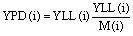
where YLL and M are the number of years lost and total mortality for each disease, and i is the respective disease. LC, ALRI and CEVH have the highest YPD, at 25 years, IHD is associated with 21 years, while COPD and CEVI have the lowest YPD, at 17 years.
Table 1 summarises all mortality rates derived from the different model configurations. The first column gives the population of the respective country. The second column shows the number of deaths per country as calculated from the ground level PM2.5 concentrations of the coarse domain, with a grid spacing of 100 km. The third column presents the respective results with aerosol concentrations as simulated in the fine resolution domain (20 km). In the next column the concentrations of PM2.5 are derived as an average value of the first three model layers below 200 m height above surface (L1 vs. L3). In all previous tests the RR parameter is calculated upon changes in PM2.5 concentrations in 1 μg m−3 steps. The fourth column shows the results where the RR parameter is calculated in concentration steps of 0.1 μg m−3, i.e. ten values for each of the values assigned in the 1 μg m−3 calculation, leading to a smoother RR distribution. Table 1 also includes the mortality rates per country based on PM2.5 concentrations from satellite estimates, both with and without observational data assimilation. The last five columns show the difference in the mortality rates due to the use of coarse vs. fine chemical model resolution ((D1-D2) × 100/D1), PM2.5 from surface vs. first three layers ((L1-L3) × 100/L1), 1 vs 0.1 μg m−3 concentration steps in the calculation of RR ((RR1-RR01) × 100/RR1), as well as a comparison between model and satellite derived mortality rates ((Mod-Sat) × 100/Mod and (Mod-SatC) × 100/Mod). The countries are sorted in descending order of deaths per year. This listing highlights the countries with more pronounced collocations of high PM2.5 concentrations and dense populations. This includes mainly eastern European countries such as Poland, Romania and Bulgaria.
Table 1. Country name, population (column 2), mortality (deaths per year) estimates per country derived from model (four configurations: columns 3–6) and satellite (two configurations: columns 7–8) PM2.5 concentrations and relative uncertainties (columns 9–13).
| COUNTRY | Population (×103) | 100 km Domain D1 | 20 km Domain D2 | 200 m (L3) lowest layer | D1 with RR 0.1µg bins | Satellite data | Satellite data ass. | (D1-D2) ×100/D1 | (L1 L 3) ×100/L1 | (RR1-RR0.1) ×100/RR1 | (Mod-Sat) ×100/Mod | (Mod-Sat_data ass.) ×100/Mod |
|---|---|---|---|---|---|---|---|---|---|---|---|---|
| Germany | 80435 | 52823 | 53708 | 53532 | 53167 | 47993 | 45991 | −1.67 | 0.33 | 1 | 9.73 | 13.49 |
| Italy | 59588 | 28423 | 30128 | 29824 | 29733 | 25650 | 27529 | −6 | 1.01 | 1.31 | 13.73 | 7.41 |
| Poland | 38575 | 26207 | 26326 | 26225 | 26019 | 27380 | 27374 | −0.45 | 0.38 | 1.18 | −5.23 | −5.21 |
| France | 62961 | 21138 | 21670 | 21385 | 21393 | 14709 | 15536 | −2.52 | 1.31 | 1.27 | 31.24 | 27.38 |
| Romania | 20299 | 17669 | 18236 | 18203 | 17994 | 19915 | 17815 | −3.21 | 0.18 | 1.35 | −10.67 | 0.99 |
| Spain | 46601 | 12871 | 13784 | 13614 | 13480 | 8783 | 9452 | −7.09 | 1.23 | 2.25 | 34.84 | 29.88 |
| Hungary | 10014 | 8844 | 8923 | 8918 | 8798 | 9077 | 8656 | −0.89 | 0.05 | 1.4 | −3.17 | 1.61 |
| Netherlands | 16632 | 8552 | 8676 | 8546 | 8596 | 6748 | 6329 | −1.45 | 1.49 | 0.93 | 21.49 | 26.37 |
| Bulgaria | 7407 | 8081 | 8259 | 8230 | 8149 | 7996 | 7237 | −2.21 | 0.34 | 1.32 | 1.87 | 11.19 |
| Czechia | 10507 | 7837 | 7954 | 7917 | 7870 | 7711 | 7648 | −1.49 | 0.46 | 1.04 | 2.02 | 2.82 |
| Belgium | 10930 | 6878 | 6978 | 6872 | 6908 | 5237 | 4994 | −1.45 | 1.52 | 1 | 24.2 | 27.71 |
| Greece | 11178 | 6615 | 6639 | 6571 | 6527 | 4402 | 4344 | −0.35 | 1.01 | 1.67 | 32.55 | 33.44 |
| Portugal | 10585 | 4660 | 5086 | 4973 | 5006 | 2876 | 2900 | −9.14 | 2.21 | 1.6 | 42.55 | 42.07 |
| Austria | 8392 | 4092 | 4127 | 4152 | 4071 | 3849 | 4068 | −0.84 | −0.61 | 1.35 | 5.5 | 0.07 |
| Slovakia | 5407 | 4088 | 4105 | 4107 | 4061 | 4073 | 4040 | −0.41 | −0.07 | 1.07 | −0.29 | 0.52 |
| Sweden⁎ | 9382 | 3605 | 3576 | 3645 | 3459 | 4064 | 3869 | 0.81 | −1.95 | 3.38 | −17.49 | −11.85 |
| Croatia | 4316 | 3115 | 3187 | 3195 | 3147 | 2796 | 2803 | −2.33 | −0.25 | 1.27 | 11.15 | 10.93 |
| Switzerland | 7831 | 2733 | 2718 | 2716 | 2673 | 2660 | 3020 | 0.57 | 0.04 | 1.67 | 0.48 | −12.98 |
| Denmark | 5550 | 2732 | 2682 | 2669 | 2641 | 2070 | 1949 | 1.83 | 0.51 | 1.51 | 21.62 | 26.2 |
| Lithuania | 3123 | 2699 | 2708 | 2736 | 2658 | 3204 | 3056 | −0.33 | −1 | 1.85 | −20.54 | −14.97 |
| Latvia | 2090 | 1825 | 1821 | 1832 | 1787 | 2096 | 1991 | 0.22 | −0.6 | 1.88 | −17.29 | −11.41 |
| Finland⁎ | 5367 | 1675 | 1694 | 1693 | 1634 | 1935 | 1818 | −1.1 | 0.08 | 3.54 | −18.42 | −11.26 |
| Ireland | 4617 | 1359 | 1360 | 1360 | 1335 | 478 | 478 | −0.05 | 0 | 1.81 | 64.19 | 64.19 |
| Norway⁎ | 4890 | 1332 | 1360 | 1362 | 1303 | 978 | 928 | −2.01 | −0.19 | 4.34 | 24.94 | 28.78 |
| Slovenia | 2051 | 1026 | 1100 | 1097 | 1085 | 925 | 990 | −7.24 | 0.25 | 1.38 | 14.74 | 8.75 |
| Estonia | 1332 | 849 | 830 | 829 | 814 | 909 | 838 | 2.2 | 0.02 | 1.92 | −11.67 | −2.95 |
| Cyprus | 1104 | 266 | 273 | 273 | 265 | 241 | 228 | −2.76 | 0.13 | 2.94 | 9.51 | 13.96 |
| Luxembourg | 508 | 197 | 207 | 202 | 205 | 150 | 142 | −4.73 | 1.97 | 0.57 | 26.83 | 30.73 |
| Malta | 412 | 135 | 142 | 138 | 139 | 21 | 10 | −5.07 | 2.9 | 2.29 | 84.89 | 92.8 |
| TOTAL | 452084 | 242326 | 248257 | 246816 | 244917 | 218926 | 217034 | −2.4% | 0.58% | 0.77% | 10.6% | 11.4% |
When comparing the number of deaths based on the pollutant concentrations from the two domains, at country level, we obtain a minor but non-linear response for the mortality estimates, with most countries exhibiting lower mortality rates in the 100 km case than at PM2.5 concentrations from the 20 km resolution domain (table 1). The reduced estimates at the coarse resolution domain over the entire domain reach –6% in Italy, –5% in Malta, −4.7% in Luxemburg, −7% in Slovenia and Spain and –9% in Portugal. In general, the countries with the largest biases cover small geographical areas, and the use of a higher resolution for PM2.5 is important to represent national boundaries. Spain is the only larger country that exhibits a significant difference from the use of the 100 km versus the 20 km resolution domain. To a lesser extent, negative biases from the coarse grid are found for Bulgaria, France, Germany, Romania, and other countries. There are four countries (Denmark, Estonia, Latvia and the United Kingdom) where the use of the 100 km yields higher mortality rates than the 20 km domain. Overall, in the EU-28, the total mortality due to particulate matter pollution reaches 242 000–248 000 depending on model configuration. The uncertainty related to the use of the course versus fine resolutions is approximately ±2.4%. In this country-based comparison, for several countries (Finland, Sweden and Norway; highlighted with an asterisk in table 1) where the use of the larger domain (with 100 km grid spacing) includes larger areas of these countries, we limit the calculations to the northern boundary of the region defined by the second domain (the dashed line in figure 1(a)).
Table 2. Premature deaths per year for each disease category (LC, ALRI, COPD, CEVH, CEVI and IHD), and totals based on modelled PM2.5 concentrations (four configurations) over Europe. MIN and MAX columns represent the range of values of the 95% confidence intervals from epidemiological data.
| DeathsDisease | MIN | D1 100 km L3 average | D2 20 km L3 average | D2 20 km L1 average | D2 20 km L3 average 0.1µg bins | MAX |
|---|---|---|---|---|---|---|
| LC | 27 825 | 37 375 | 38 683 | 39 250 | 37 875 | 48 905 |
| ALRI | 22 517 | 34 265 | 35 787 | 36 466 | 35 009 | 47 678 |
| COPD | 34 275 | 49 537 | 50 979 | 51 561 | 50 108 | 65 757 |
| CEVH | 26 472 | 44 780 | 45 923 | 46 332 | 45 215 | 63 657 |
| CEVI | 37 337 | 64 251 | 65 477 | 65 947 | 64 387 | 91 327 |
| IHD | 211 477 | 305 316 | 310 343 | 312 175 | 306 325 | 400 622 |
| ALL | 359 903 | 535 524 | 547 192 | 551 731 | 538 919 | 717 946 |
We perform the same country-based analysis by using PM2.5 concentrations at ground level (L1) and concentrations averaged over the near-surface layer of approximately 200 m (L3) to test possible differences in the model results in view of the vertical exchange processes. The use of first layer or 200 m layer PM2.5 concentrations yields statistically insignificant differences in mortality estimates, with most of the countries exhibiting uncertainties of less than 1% (0.58%). The use of the ground level concentrations leads, in general, to slightly higher mortality rates related to the slightly higher PM2.5 levels at the surface compared to the 200 m average concentration.
We also compare the mortality estimates as derived using RR calculations based on 1 and 0.1 μg m−3 concentrations bins. The calculation of RR in 1μg m−3 bins yields higher mortality rates than the RR0.1, with differences reaching 2.9% over Cyprus and 3.5% over Finland, 3.3% over Sweden and 4.3% over Norway. However, in total over the EU-28, the differences in the annual number of deaths from particulate matter pollution, driven by the resolution of the RR calculation, are within 0.8%.
We additionally calculated mortality rates based on PM2.5 concentrations derived from satellite observations, with and without assimilation of ground observational data, as described in van Donkelaar et al (2016). In general, satellite-derived aerosol levels yield approximately 10% lower mortality rates over the EU-28. The use of the assimilated PM2.5 values leads to improved agreement between the satellite-based mortality results and the results of our regional model, which in the present application does not use data assimilation. Apart from Germany, in the top ten countries and in terms of deaths per year rates, the data assimilation process in the satellite output brings satellite mortality rates closer to our model results by either reducing or increasing the non-corrected satellite driven estimates. This is particularly evident in six of the top seven countries, which account for almost half of the premature deaths in EU-28 (Italy, Poland, France, Romania, Spain, and Hungary).
For a domain-wide analysis, we mask the mortality estimates delivered from the coarse domain to produce only mortality rates for the grid cells included in the fine domain in order to compare similar areas. From this comparison, as summarised in table 2, over the entire domain (the European continent, including parts of west Asia and North Africa) the deaths due to air pollution reach over half a million people per year. The different configuration modes slightly alter the mortality estimates over the domain, with values varying from 535 000 to 552 000 deaths per year, while the uncertainties from epidemiological data lead to a range of 360 000–718 000 annual deaths (95% confidence interval).
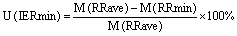
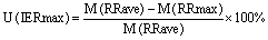
In figure 6 we summarise all uncertainties in mortality rates that can be attributed to model configuration (domain grid spacing–grey columns; vertical level–yellow columns; and RR concentration bins–green columns) and the uncertainties introduced by the range of the epidemiological data that define the relative risk of disease, shown by the minimum (light blue) and maximum (light red) values of RR (95% confidence interval). The uncertainties (U) are calculated, per disease and in total, as follows.

Figure 5. Annual premature mortality rates for EU-28 countries derived from PM2.5 concentrations from the model (blue columns), satellite estimates without correction through data assimilation (orange columns) and satellite estimates with observational data assimilation (grey columns).
Download figure:
Standard image High-resolution image
Figure 6. Uncertainties in mortality estimates related to model configuration (domain grid spacing in grey, level of PM2.5 concentration in yellow), RR concentrations step (in green) and the 95% confidence interval in IER functions (lower range in blue and upper range in red) for each disease and in total.
Download figure:
Standard image High-resolution image95% uncertainty interval lower IER:
95% uncertainty interval higher IER:
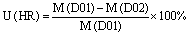
Horizontal resolution (HR) uncertainty:
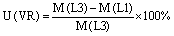
Vertical resolution (VR) uncertainty:
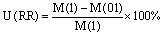
RR concentration step (RR) uncertainty:
where M is the mortality estimate for each case, D01 and D02 are respectively the coarse and fine grid domains, L3 and L1 are the averaged three first levels and ground level model results, and 1 and 01 are the mortality estimates from the calculation of the relative risk in the 1μg m−3 and 0.1 μg m−3 concentration bins.
Figure 6 illustrates that the uncertainties due to domain configurations vary from −3.5% to 2.1% for LC, −4.4% to 2.2% for ALRI, −2.9% to 1.7% for COPD, −2.6% to 1.5% for CEVH, −1.9% to 1.7% for CEVI and −1.6% to 1.3% for IHD, averaging over all diseases to −2.2% to 1.5%, with the negative values attributed to the impact of higher resolution and the positive values attributed to the impact of the smaller concentrations size bin for the calculation of RR (0.1 μg m−3 versus 1 μg m−3). The uncertainties from the use of the 95% confidence interval (minimum and maximum values) of RR reach +25% to −31% for LC, +34% to −39% for ALRI, 31% to −33% for COPD, 41% to −42% for CEVH and CEVI, ±31% for IHD, and an average IER uncertainty between +32.8% and −34.1%. We conclude that the domain-wide average differences in mortality rates that can be attributed to model configuration are significantly smaller than the uncertainties of the epidemiological data that define the relative risk of disease within the 95% confidence interval.
5. Conclusions
We performed several sensitivity tests to calculate mortality rates over Europe. We used a regional coupled air quality model (WRF-Chem) with two domains at 100 km and 20 km grid resolutions, respectively, to simulate PM2.5 concentrations and, in turn, the number of premature deaths per year attributed to aerosols for IHD, CEV, LRIs such as pneumonia, COPD and LC. The base mortality rates are calculated based on ground PM2.5 concentrations for both domains. We also used 200 m above ground average PM2.5 to account for possible shortcomings of model simulations related to near-surface exchange processes. Additionally, we calculated the relative risk factor in 1μg m−3 and 0.1 μg m−3 concentration bins for a smoother distribution of relative risk (RR).
The mortality rates differ by 2.4% due to horizontal resolution of the model configuration, by 0.6% due to the vertical distribution of PM2.5, and by 0.8% due to the resolution of RR. Estimates based on PM2.5 concentrations derived from satellite data are within 10% of the model results. The use of data assimilation in the satellite estimates brings mortality rates for most of the countries having high death rates closer to the model results. On the other hand, the 95% confidence intervals of the IER functions for these diseases give rise to statistical uncertainties in the estimates within about ± 30%. These results indicate that the uncertainties of mortality estimates are dominated by the estimated response of population to air pollution, derived from epidemiological data, rather than the representation of annual mean PM2.5 values by air quality models and/or observations.
Acknowledgments
The computational resources and support were provided by the European Union Horizon 2020 research and innovation programme VI-SEEM project under grant agreement 675121. The near-surface PM2.5 distributions based on satellite data can be accessed at the Atmospheric Composition Analysis Group of the Department of Physics and Atmospheric Science, Dalhousie University, (http://fizz.phys.dal.ca/~atmos/martin/?page_id=140). The aerosol measurements are derived from the AirBase European-wide air quality database hosted by the European Environmental Agency (EEA) that contains validated air quality monitoring information for more than 30 participating countries throughout Europe (available at http://aidef.apps.eea.europa.eu, www.eea.europa.eu/data-and-maps/). We acknowledge the use of the anthropogenic emission datasets downloaded from http://edgar.jrc.ec.europa.eu/htap_v2/. The emissions were prepared in the framework of the Task Force on Hemispheric Transport of Air Pollution (TF-HTAP) organised in 2005 under the auspices of the UNECE Convention on Long-range Transboundary Air Pollution (LRTAP Convention). The authors would also like to thank the two anonymous referees for their reviews and constructive comments.