

Abstract
We use the 100-member Grand Ensemble with the climate model MPI-ESM to evaluate the controllability of mean and extreme European summer temperatures with the global mean temperature targets in the Paris Agreement. We find that European summer temperatures at 2 °C of global warming are on average 1 °C higher than at 1.5 °C of global warming with respect to pre-industrial levels. In a 2 °C warmer world, one out of every two European summer months would be warmer than ever observed in our current climate. Daily maximum temperature anomalies for extreme events with return periods of up to 500 years reach return levels of 7 °C at 2 °C of global warming and 5.5 °C at 1.5 °C of global warming. The largest differences in return levels for shorter return periods of 20 years are over southern Europe, where we find the highest mean temperature increase. In contrast, for events with return periods of over 100 years these differences are largest over central Europe, where we find the largest changes in temperature variability. However, due to the large effect of internal variability, only four out of every ten summer months in a 2 °C warmer world present mean temperatures that could be distinguishable from those in a 1.5 °C world. The distinguishability between the two climates is largest over southern Europe, while decreasing to around 10% distinguishable months over eastern Europe. Furthermore, we find that 10% of the most extreme and severe summer maximum temperatures in a 2 °C world could be avoided by limiting global warming to 1.5 °C.
Export citation and abstract BibTeX RIS

Original content from this work may be used under the terms of the Creative Commons Attribution 3.0 licence.
Any further distribution of this work must maintain attribution to the author(s) and the title of the work, journal citation and DOI.
1. Introduction
Recent decades have been marked by an increasing number of extremely warm summers over the European continent (Schär et al 2004, Christidis et al 2014), and this rising tendency, largely attributed to anthropogenic climate change, is expected to be accentuated under further global warming (Stott et al 2004, Meehl and Tebaldi 2004, Christidis et al 2014, Vautard et al 2014). In the framework of the Paris Agreement, it is crucial to evaluate which of the risks and impacts of climate change would be reduced by limiting global warming to 1.5 °C (hereafter 1.5 °C target) in contrast to by limiting warming to 2 °C (hereafter 2 °C target). Here we examine to what extent the most extreme European summer temperatures at 2 °C of global warming could be avoided in a 1.5 °C warmer world. In other words, we examine to what extent extreme European summer temperatures could be controlled by limiting global warming to the global mean temperature limits of the Paris Agreement. To evaluate the controllability of European summer temperatures with global mean temperature limits it is necessary to robustly characterize the irreducible uncertainty that arises from chaotic internal variability (Sriver et al 2015, Hawkins et al 2016). For this purpose, we use a state-of-the-art tool to sample internal variability: the 100-member Max Planck Institute Earth System Model (MPI-ESM) Grand Ensemble (Bittner et al 2016, Hedemann et al 2017, Suárez-Gutiérrez et al 2017).
Summer monthly mean and daily maximum temperatures at 2 °C of global warming are projected to become around 1 °C higher over Europe than at 1.5 °C of warming (Schleussner et al 2016, Perkins-Kirkpatrick and Gibson 2017, King and Karoly 2017, Sanderson et al 2017). Sanderson et al (2017) and Wehner et al (2017) also find differences of around 1 °C between 20 year return levels of maximum temperatures at 1.5 °C versus at 2 °C of global warming. These studies are based on climate modelling experiments of different nature: the Coupled Model Intercomparison Project phase 5 (CMIP5) multi-model ensemble (Schleussner et al 2016, Perkins-Kirkpatrick and Gibson 2017, King and Karoly 2017), and ensemble-experiments such as the Half a Degree Additional warming, Prognosis and Projected Impacts project (HAPPI; Mitchell et al 2017) atmosphere-only runs (Wehner et al 2017), and the Community Climate ten-member CESM1 ensemble (Sanderson et al 2017).
A key factor in evaluating the differences between the climates for the two targets is to consider the magnitude of the response in the Earth's climate to half a degree more of warming relative to the signal of internal variability. For this purpose, large ensembles of simulations based on the same coupled climate models (like the experiments described in Deser et al 2012, Kay et al 2015, Rodgers et al 2015, Fyfe et al 2017, Sanderson et al 2017 and Suárez-Gutiérrez et al 2017) are the best available tools, because they provide unambiguous characterisations of the simulated internal variability in a changing climate without being confounded by different model configurations. The MPI-ESM Grand Ensemble has 100 independent realizations, which start from different times of a pre-industrial control run but are driven by the same external forcings, and is currently the largest existing ensemble from a fully-coupled Earth System Model. The large size of the ensemble is a crucial requirement to robustly sample internal variability and to empirically evaluate the statistical significance of changes. An ensemble size of 100 simulations under the same forcing conditions allows 1-in-100-years events to occur on average every simulated year, which provides the large samples of extreme events under different warming conditions that are necessary for the purpose of our study.
We use the MPI-ESM Grand Ensemble not only to evaluate average changes in summer monthly mean, block maximum, and extreme temperatures, but also to quantify the irreducible uncertainty in European summer temperatures that arises through internal variability. We evaluate the controllability of European summer temperatures with global temperature targets by quantifying the distinguishability of European summer months at 2 °C of global warming with respect to those in a 1.5 °C warmer world. We also quantify for the first time changes in the magnitude of extreme summer temperature events with return periods of up to 500 years.
2. Data and methods
We use transient climate simulations from the 100-member MPI-ESM Grand Ensemble under historical, RCP2.6 and RCP4.5 forcing conditions. The Grand Ensemble uses the model version MPI-ESM1.1 in the low resolution (LR) configuration, with resolution T63 and 47 vertical levels in the atmosphere (Giorgetta et al 2013) and 1.5° resolution and 40 vertical levels in the ocean (Jungclaus et al 2013). MPI-ESM1.1 has an equilibrium climate sensitivity of 2.8 °C and a transient climate response of 1.57 °C, values that are slightly below the values for the CMIP5 version of MPI-ESM (Flato et al 2013). Each of the 100 realizations in the ensemble is based on the same model physics and parametrizations, and is driven by the same external forcings. The realizations differ only in their initial climate state, taken from different points of the model's pre-industrial control run.
MPI-ESM-LR has a relatively low resolution, comparable to most of the models in the CMIP5 experiment, which can influence the model's ability of simulating small-scale processes and affect the reliability of our projections. However, we find that the MPI-ESM Grand Ensemble offers an adequate representation of the observed estimate of internal variability in global mean temperatures and European summer temperatures. We present a detailed model evaluation in the supporting information (SI) available at stacks.iop.org/ERL/13/064026/mmedia, in which we find a slight overestimation of the frequency of colder than average summer months in the ensemble simulations that may be partially caused by biases in precipitation variability (SI figures S1, S2 and S3). Observational data from the HadCRUT4.5 (Morice et al 2012, Osborn and Jones 2014) and the CRUTEM4.6 (Jones et al 2012) datasets are used for comparisons to current climate conditions.
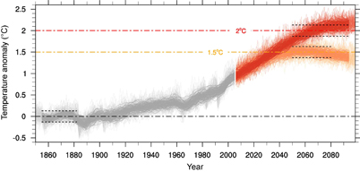
Figure 1. Global mean surface temperature (GMST) in the MPI-ESM Grand Ensemble. Time series of annually averaged GMST anomalies (coloured thin lines) and centered decadal-averaged GMST anomalies (coloured thick lines) for the period 1850–2099, simulated by the MPI-ESM Grand Ensemble. Simulations are historical runs for the period 1850–2005 (gray lines), and RCP2.6 (orange lines) and RCP4.5 (red lines) for the period 2006–2099. The black dashed lines show the periods of sampling for each warming level and the standard deviation of GMST from the long-term warming levels for pre-industrial and warming targets of 1.5 °C and 2 °C.
Download figure:
Standard image High-resolution imageGlobal mean surface temperature (GMST) is defined as the annually averaged, global mean, near-surface 2 m air temperature anomaly. European monthly mean summer temperature (EuST) is defined as the monthly averaged 2 m air temperature anomaly for the summer months (JJA), averaged over the land-only grid cells in the region defined by the [10°W–50°E, 35–60°N] latitude-longitude domain. Ideally, we would use daily temperatures to capture the amplitude of internal variability more precisely. However, monthly frequency is the highest output frequency in the Grand Ensemble simulations. We also use the summer maximum value of daily maximum temperature (EuSTXx) as the block maximum temperature anomaly reached each summer at each grid cell averaged over the land-only grid cells in the same domain. All anomalies are calculated with respect to the pre-industrial conditions defined by the period 1851–1880. Observed temperature anomalies are transformed to anomalies with respect to pre-industrial levels following the estimates in Hawkins et al (2017).
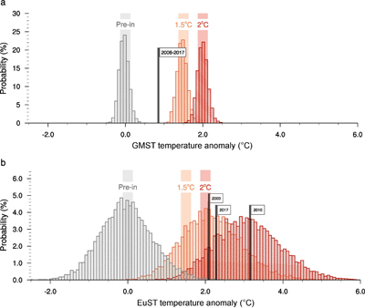
Figure 2. Probability distributions at different global warming levels. (a) Probability distribution of GMST anomalies for pre-industrial conditions (gray), and for global warming levels of 1.5 °C (orange) and 2 °C (red) above pre-industrial levels, simulated by the MPI-ESM Grand Ensemble. The shaded areas indicate the range of ± one standard deviation of GMST around the mean state of 0 °C (gray), 1.5 °C (orange) and 2 °C (red). Each distribution has a sample size of around 3000 simulated years. The black reference line marks the observed decadal-average GMST anomaly for 2008–2017 from HadCRUT4 data. (b) Probability distribution of EuST anomalies for pre-industrial conditions (gray), and for global warming levels of 1.5 °C (orange) and 2 °C (red) above pre-industrial conditions, as in (a). Each distribution has a sample size of around 9000 summer months. The black reference lines mark the observed EuST monthly mean anomaly for August 2003, August 2017 and July 2010 from CRUTEM4 data. Bin size is 0.075 °C; frequencies are normalized to unity and translated to percentage.
Download figure:
Standard image High-resolution image
Figure 3. Mean temperatures and temperature variability at different global warming levels. (a) Average monthly mean temperature anomaly at 1.5 °C of global warming. (b) Spread in monthly mean temperature anomalies at 1.5 °C of global warming, measured as the difference between the 97.5th and 2.5th percentiles. (c) Average monthly mean temperature anomaly at 2 °C of global warming. (d) Spread in monthly mean temperature anomalies at 2 °C of global warming, as in (b). (e) Difference in average monthly mean temperature anomaly at 2 °C of global warming minus at 1.5 °C of global warming. (f) Difference in the spread in monthly mean temperature anomalies at 2 °C of global warming minus at 1.5 °C of global warming, as in (b). (g) Summer months at 2 °C of global warming with temperatures that could be distinguishable from those at 1.5 °C based on the areal overlap between the two distributions. (h) Summer months at 2 °C of global warming with temperatures that could be distinguishable from those at 1.5 °C based on the percentage of months at 2 °C of warming above the 95th percentile in the 1.5 °C distribution.
Download figure:
Standard image High-resolution image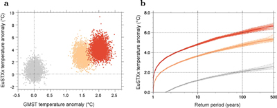
Figure 4. European summer maximum value of daily maximum temperature (EuSTXx) at different global warming levels. (a) EuSTXx anomalies against GMST anomalies for pre-industrial conditions (gray), and for global warming levels of 1.5 °C (orange) and 2 °C (red) above pre-industrial conditions, simulated by the MPI-ESM Grand ensemble. (b) Return levels of EuSTXx summer block maxima against their return period, represented by the thick solid lines in gray for pre-industrial conditions, in orange for global warming levels of 1.5 °C and in red for 2 °C above pre-industrial conditions. Uncertainty in these return levels is estimated by bootstrap-resampling with replacement. The coloured thin lines represent 1000 individual bootstrap estimates; the coloured dashed lines represent the 95% confidence intervals.
Download figure:
Standard image High-resolution imageWe construct representative samples of the quasi-stationary climate conditions at 1.5 °C and 2 °C of global warming from transient climate simulations with a time-slice method that is similar to the methods used in Schleussner et al (2016) or King and Karoly (2017). We select years of 0 °C, 1.5 °C, and 2 °C of global warming with respect to pre-industrial levels from all historical, RCP2.6, and RCP4.5 100-member simulations from the MPI-ESM Grand Ensemble. Global mean temperatures deviate from the long-term mean state on year-to-year timescales due to the effect of internal variability. Therefore, we calculate centered decadal-averaged GMST to robustly define global warming levels. We define years of 0 °C of global warming as those years in which the centered decadal-averaged GMST is in the range of 0 °C plus-minus one standard deviation of GMST, 0.13 °C. Similarly, for 1.5 °C and 2 °C of global warming above pre-industrial levels we select years in which the centered decadal-averaged GMST is in the range of 1.5 °C±0.13 °C and 2 °C±0.13 °C, respectively.
Based on this assumption of quasi-stationarity, we are able to calculate well-defined return levels of maximum daily temperature anomalies for extreme events with return periods of up to 500 years based on the probability distributions of spatially averaged EuSTXx. The high ensemble resolution provides large enough samples of extreme events, with 3000 simulated years for each climate conditions, that allow us to empirically calculate probability distributions and eliminate the need to parametrise the tails of the distributions with extreme value statistics. We calculate the return period of any given return level as the inverse of the probability of exceedance of this return level per year. We obtain this probability of exceedance directly as one minus the cumulative probability of the given return level.
3. Results
We evaluate three sets of 100 transient climate simulations under historical, RCP2.6 and RCP4.5 forcings from the MPI-ESM Grand Ensemble. Figure 1 illustrates the characterization of the global warming levels analysed here. Within the 21st century, around half of the ensemble members show GMST projections that remain below the 2 °C warming target for the RCP4.5 scenario, while most of the GMST projections following the RCP2.6 scenario are in agreement with the 1.5 °C warming target. To achieve a sample size of around 3000 simulated years for each climate, we choose only simulated years within the periods marked by the black dashed lines in figure 1.
3.1. European summer monthly mean temperatures
The empirical probability distributions of GMST for the years selected from the Grand Ensemble simulations show that the three samples describing pre-industrial climate conditions and the climates for the two targets are significantly distinguishable from each other (figure 2(a)). The distribution of GMST for pre-industrial conditions, with a width of around 0.9 °C, presents no overlap with either the 1.5 °C or the 2 °C distributions. The two target distributions overlap over 5% of their area and have a width of around 1 °C. Using a narrower range in decadal-averaged GMST for defining each climate reduces the sample size of the distributions, but does not substantially influence our results.
Whereas the climates for the two warming targets are distinguishable at the global level, European summer temperatures have substantially larger internal variability than global mean temperatures. The probability distributions of summer monthly mean temperature anomalies for the selected years describing the two target climates present a width more than four times larger than the GMST distributions (figure 2(b)). In contrast to the GMST distributions, and due to the large influence of internal variability, all three distributions of European summer temperatures for different warming levels present some fraction of areal overlap. This overlap is largest when comparing the two target climates, with a 60% areal overlap between the EuST probability distributions at 1.5 °C and at 2 °C.
With respect to the relative GMST distributions, the EuST distributions for both warming targets are also shifted towards higher mean temperature anomalies. The probability distribution of EuST is centered around 2 °C anomalies at 1.5 °C of global warming, and for 2 °C of global warming is centered around anomalies of 3 °C, indicating a pattern of regional amplification of global warming over Europe that is in line with previous expectations (IPCC 2013).
The two highest observed European summer monthly mean temperatures in July 2010 and August 2017 are marked in figure 2(b) for comparison, as well as the value for August 2003. The estimates for 2003 and 2017 are comparable to the average European summer month in a 1.5 °C warmer world, and also comparable to summer months in the upper tail of the pre-industrial distribution. This result is consistent with previous findings that project the 2003 summer temperatures to become commonplace around the 2040s (Stott et al 2004). On the other hand, the 2010 value is comparable to the average summer month in a 2 °C warmer world. This result indicates that, under 2 °C of global warming, every other European summer month would be warmer than the warmest summer month on record in current climate conditions; while the other half of European summer months in a 2 °C world would be more similar to current climate conditions. However, the 60% of areal overlap between the two target distributions indicates that less than half of the European summer months in a 2 °C world, four months out of every ten, would be distinguishable from those in a 1.5 °C world.
Figure 3 illustrates these results locally, presenting differences in mean temperatures and in temperature variability as well as distinguishability between the two warming limits per grid cell. Mean temperature differences are around 1 °C, consistent with the results shown by King and Karoly (2017) and Sanderson et al (2017), and largest over the Mediterranean region (figure 3(e)). However, the temperature variability, measured as the width of the local probability distributions between the 97.5th and 2.5th percentiles, is very large over these regions (figures 3(b) and (d)). This irreducible spread caused by internal variability of up to 10 °C is much larger than the average temperature changes. However, the change in variability in European summer temperatures is relatively small in comparison with the mean temperature changes and is localized over central-northern Europe (figure 3(f)). This pattern of change in variability, shown here as the difference in spread, is also present when variability changes are portrayed as ratios (figure S4 in the SI).
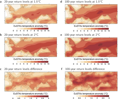
Figure 5. Return levels of summer block maximum daily temperatures at different global warming levels. (a) Daily maximum temperature anomalies for events with 20-year return periods at 1.5 °C of global warming. (b) Daily maximum temperature anomalies for events with 20-year return periods at 2 °C of global warming. (c) Daily maximum temperature anomalies for events with 20-year return periods at 2 °C of global warming minus at 1.5 °C of global warming. (d) Daily maximum temperature anomalies for events with 100-year return periods at 1.5 °C of global warming. (e) Daily maximum temperature anomalies for events with 100-year return periods at 2 °C of global warming. (f) Daily maximum temperature anomalies for events with 100-year return periods at 2 °C of global warming minus at 1.5 °C of global warming.
Download figure:
Standard image High-resolution image
Figures 3(g) and (h) show how often European summer months at 2 °C of global warming could be distinguishable from those at 1.5 °C of warming for each grid cell. We define the distinguishability between the two target climates as the percentage of summer months in a 2 °C world that could not be part of the temperature distribution of the 1.5 °C world. For figure 3(g), we base this estimate of distinguishability between the two climates on the areal overlap between the two temperature distributions at grid-cell level. This distinguishability is largest over Southern Europe, with a maximum of around 35% distinguishable summer months, and decreases to around 10% for Eastern Europe. We also include a second, more conservative measure of distinguishability in figure 3(h), based on the percentage of summer months in a 2 °C world that present EuSTs larger than the 95th percentile in the EuST distribution at 1.5 °C of warming. This measure of distinguishability yields values of around 5%–20% months with distinguishable mean temperatures. For both measures, we find the minimum distinguishability between the two climates over eastern Europe, where summer temperature variability is largest.
3.2. Return levels in European summer maximum temperatures
In this section we evaluate how the return levels of extreme European summer temperatures change under global warming. We base our analysis on block maximum values of daily maximum temperature (EuSTXx) simulated by the MPI-ESM Grand Ensemble, shown in figure 4(a) against simultaneous global mean temperatures for the three sampled climate conditions. EuSTXx anomalies exhibit large variability, with a spread of more than 4 °C. EuSTXx anomalies are centered around 3 °C in a 1.5 °C warmer world, and around 4 °C in a 2 °C warmer world. The EuSTXx distributions for 1.5 °C and 2 °C of warming present an areal overlap of 70% (not shown), indicating that only three out of every ten of the summer maximum temperatures in a 2 °C warmer world could be distinguishable from those in a 1.5 °C world. Due to this large overlap and the large variability in block maximum daily maximum temperatures, only 10% of the most extreme EuSTXx values at 2 °C of warming would be out of reach in a 1.5 °C warmer world (with 99% confidence).
The return levels of summer maximum daily maximum temperature anomalies for events with return periods from 1 to 500 years are presented in figure 4(b) for the three sampled climate conditions. 2 °C events, which have return periods of around 100 years under pre-industrial conditions, are projected to occur every one to two years in both target climates. 10-year return period events present values of around 3.5 °C in a 1.5 °C warmer world and of around 5 °C in a 2 °C warmer world. This difference of 1 °C to 1.5 °C in return levels of extreme summer temperatures between the two target climates is roughly maintained for increasingly longer return periods. For 500-year return periods, we find return levels that reach values of almost 7 °C at 2 °C of global warming and of around 5.5 °C at 1.5 °C of global warming. We reach similar results by basing this analysis on the summer minimum value of daily minimum temperatures (EuSTXn; SI figure S5).
20-year return levels of EuSTXx anomalies present a maximum over south-eastern Europe and are generally largest in southern Europe for both target climates (figures 5(a) and (b)). The difference in 20-year return levels between the two target climates is also largest in southern Europe, with values around 1.5 °C (figure 5(c)), overlapping with the region of largest mean temperature increase in figure 3(e). Similarly, 100-year return levels also present a maximum over south eastern Europe (figures 5(d) and (e)). In contrast to events with shorter return periods, extreme events with return periods of 100 to 500 years (not shown) present differences between the two target climates that are largest in central Europe, over the regions where we find the largest increase in temperature variability in figure 3(f) (figure 5(f)).
4. Summary and conclusions
We use the state-of-the-art MPI-ESM Grand Ensemble to evaluate the controllability of monthly mean, block maximum, and extreme European summer temperatures under the global warming limits of the Paris Agreement. We find that at 2 °C of global warming, one out of every two European summer months is projected to be warmer than ever observed in our current climate. We find European summer monthly mean temperature differences of around 1 °C between the 2 °C and the 1.5 °C warmer worlds, in line with previous results by Schleussner et al (2016), Perkins-Kirkpatrick and Gibson (2017), King and Karoly (2017), and Sanderson et al (2017). We also find differences of around 1 °C in maximum daily temperature anomalies for extreme events with return periods of up to 500 years, which reach values of almost 7 °C at 2 °C of global warming and of around 5.5 °C at 1.5 °C of global warming. For 20-year return period events these differences are consistent with the differences in 20-year return levels shown by Sanderson et al (2017) and Wehner et al (2017), reaching values of around 1.5 °C. These differences in 20-year return levels are largest in southern Europe, over the regions where we find the largest mean temperature increase. For events with return periods of 100–500 years these differences reach values of more than 2.5 °C and are largest in central Europe, over regions where we find the largest temperature variability increase.
Our results indicate that due to the irreducible uncertainty in European summer temperatures caused by internal variability, only 40% of the European summer monthly mean temperatures in a 2 °C warmer world would be distinguishable from those in a 1.5 °C warmer world. This distinguishability between the two climates is largest over southern Europe, and decreases to around 10% over eastern Europe. Furthermore, we find that only 10% of the most extreme summer maximum temperatures in a 2 °C world would be avoided at 1.5 °C of global warming. However, although only 10% of the most extreme temperatures could be avoided, these events would correspond to the most extreme and severe heat waves, the ones with the most critical consequences.
Although these results may be subject to uncertainties inherent to any single-model study as well as to the relatively low resolution of MPI-ESM-LR, we believe that the concepts and methods at the core of our analysis can serve as blueprint for future studies with focus on other regions and phenomena. Our findings highlight the limited controllability of the amplitude of extreme temperature events at regional levels by establishing global mean temperature limits and emphasize the importance of considering the irreducible uncertainty introduced by chaotic internal variability to evaluate the impacts of climate change.
Acknowledgments
This research was supported by the Max Planck Society for the Advancement of Science and by the German Ministry of Education and Research (BMBF) under the MiKlip project FLEXFORDEC (Grant number 01LP1519A). C L acknowledges funding from the German Science Foundation (DFG) through the Cluster of Excellence 'Integrated Climate System Analysis and Prediction (CLISAP)' (Grant number EXC177). This research also contributes to the JPI Climate-Belmont Forum project InterDec. We acknowledge Luis Kornblueh, Jürgen Kröger and Michael Botzet for producing the historical, RCP2.6 and RCP4.5 MPI-ESM Grand Ensemble simulations, and the Swiss National Computing Centre (CSCS) and the German Climate Computing Center (DKRZ) for providing the necessary computational resources. We would also like to acknowledge the groups that developed and facilitated the observational compilations used in our study: the Climatic Research Unit (University of East Anglia) in conjunction with the Hadley Centre (UK Met Office). We thank one anonymous reviewer and Francis Zwiers for their insightful and constructive comments on our manuscript. We also thank Frank Sienz and Christopher Hedemann for their helpful comments and remarks. Scripts used in the analysis and other supporting information that may be useful in reproducing the authors work are archived by the Max Planck Institute for Meteorology and can be obtained by contacting publications@mpimet.mpg.de.