Evaluating the use of biomass energy with carbon capture and storage in low emission scenarios

Naomi E Vaughan; Clair Gough; Sarah Mander; Emma W Littleton; Andrew Welfle; David E H J Gernaat; Detlef P van Vuuren

doi:10.1088/1748-9326/aaaa02

Introduction

The Paris Agreement on Climate Change focuses on limiting global average temperature increase to well below 2 °C above pre-industrial level with aspirations to limit warming to 1.5 °C (UNFCCC 2015). Integrated assessment models (IAMs) are used to analyse mitigation scenarios that are compatible with atmospheric concentrations of greenhouse gases associated with different probabilities of reaching these temperature targets (Clarke et al 2014, UNEP 2016). The purpose of IAMs is to explore possible futures and uncertainties associated with those futures. They do so by providing information on alternative low-cost emission scenarios subject to various model assumptions, such as physical constraints on energy systems and timing of international climate policy; they are not intended to provide predictions of the future.

From the pathways provided by IAMs in recent years, a default mitigation strategy emerges that would be consistent with the Paris Agreement's targets: pathways show an early peak in emissions, followed by rapid emission reductions and finally a period of net negative emissions (Fuss et al 2014, Anderson and Peters 2016). These net negative emissions refer to active removal of carbon dioxide from the atmosphere, achieved by introducing new carbon sinks on a large scale (Rockström et al 2016). The advantages of using negative emissions as part of a mitigation strategy is that they can: (1) somewhat alleviate the need for very rapid near-term emission reductions and (2) compensate emissions from hard to abate sectors.

IAMs have regularly incorporated negative emissions using approaches such as afforestation (establishing new forests on previously deforested land) or biomass energy with carbon capture and storage (BECCS) (Azar et al 2013, Bauer et al 2017). Other options include, for instance, direct air capture with storage of CO₂ and enhanced weathering (some individual studies have looked into these options) (e.g. Sanz-Perez et al 2016). Although none of these approaches is widely established, BECCS is the most prominent in the IAM scenarios (Fuss et al 2014). BECCS offers the advantages to modelled scenarios of providing a non-fossil fuel energy conversion service and a potentially cost-effective approach to achieving negative emissions (Boysen et al 2017). Biomass feedstocks (from residues and dedicated energy crops) are utilised with CCS in IAMs in three main ways: (1) electricity generation, (2) hydrogen production and (3) liquid fuels (Bauer et al 2017).

The social, economic and political feasibility of achieving negative emissions at a large scale have been called into question by a number of authors (e.g. Larkin et al 2017, Rockström et al 2016, Anderson and Peters 2016). An expert assessment of explicit and implicit assumptions associated with how IAMs model negative emissions, concluded that high uncertainties remain regarding the potential for large scale (global net) negative emissions from BECCS (Vaughan and Gough 2016). Following the Paris Agreement, additional model runs have been conducted to explore the implications for reaching the 1.5 °C target. Here, we further unpack the assumptions for BECCS with respect to 2 °C and 1.5 °C, adopting a more detailed quantitative approach. The aim of this paper is to clearly set out the assumptions presented in selected IAM scenarios relating to negative emissions in the context of current understanding and considering the feasibility and issues associated with achieving levels of BECCS presented.

Methods

In this paper, we look into the detailed assumptions and results of a single IAM, the IMAGE model framework, to learn more about the required implementation strategy of the default mitigation response. IMAGE has 26 regions and countries (supplementary table S1 available at stacks.iop.org/ERL/13/044014/mmedia). The IMAGE framework includes BECCS for electricity and hydrogen generation and in industry. It can also generate negative emissions from afforestation through reforestation of degraded forest areas. It uses a spatially explicit representation of the associated land use change. It does not currently include alternative forms of carbon dioxide removal such as direct air capture with storage or enhanced weathering. Here, four scenarios from the IMAGE model are presented (table 1). In this paper the reference scenario is the IMAGE implementation of SSP2, reflecting a 'middle of the road' narrative of future global socio-economic trends as part the Shared Socio-economic Pathways (SSPs, the IMAGE implementation is described by van Vuuren et al 2017a) without climate policy action. The IMAGE model is one of six IAMs that have originally implemented the SSP framework within which the social, economic, and environmental sustainability implications of climate change mitigation and adaptation are assessed (Riahi et al 2017, Bauer et al 2017). The three low emission scenarios used in this study assume some delays in global mitigation efforts, with full global cooperation commencing in 2030 (so-called SPA2) (Riahi et al 2017). The low emission scenario names reflect the probability of reaching particular temperature limits (table 1), i.e. '1.5 °C–66%' has a 66% chance of limiting global warming by the end of the century to 1.5 °C above pre-industrial. A key driver of the uncertainty in the amount of global warming resulting from particular emissions is the response of the carbon cycle. IMAGE uses the LPJml model (Sitch et al 2003, Bondeau et al 2007) in combination with the MAGICC climate emulator model to represent the carbon cycle and climate system. While LPJml is a state-of-the-art carbon cycle model, MAGICC is an emulator that has been shown to simulate similar carbon cycle and climate dynamics over time to state-of-the-art Earth System Models (Jones et al 2016). The wider energy system changes within the four scenarios are presented in supplementary figures S1 and S2.

Table 1. The IMAGE scenarios used in this paper. All are based on the IMAGE implementation of SSP2 (van Vuuren et al 2017a). The mitigation scenarios are implemented via a universal GHG price assuming some delay (SPA2) (see Riahi et al 2017, van Vuuren et al 2017b).

Scenario name	Radiative forcing (W m⁻²)	Probability	Median temperature rise in 2100 (°C above pre-industrial)
Reference	6.5	—	3.7
2.0 °C–50%	3.4	50%	2.0
2.0 °C–66%	2.6	66%	1.6
1.5 °C–66%	2.0	66%	1.3 with overshoot

Figure 1. Refer to the following caption and surrounding text. — **Figure 1.** Mitigation of CO₂ relative to the Reference scenario for the three low emission scenarios. The thick black line shows total CO₂ emissions in the Reference scenario. The lowest thin black line shows total CO₂ emission for each scenario (a) 2 °C–50%, (b) 2 °C–66% and (c) 1.5 °C–66% in each panel. The shaded areas show the emission reductions from each sector: energy demand; energy supply; agriculture, forestry and other land use (AFOLU); fossil fuels with CCS; and biomass energy with CCS. This figure is comparable to figure 9 in Fricko *et al* 2017.
Download figure:
Standard image High-resolution image

Results and discussion

The scenarios illustrate one set of possible solutions to achieving the temperature limits of 1.5 °C and 2 °C (figure 1). A wider suite of possible solutions are presented in the SSPs (Riahi et al 2017, Bauer et al 2017). The role of BECCS in delivering the emissions reductions compared to the reference scenario is clear in all three low emission scenarios, making its greatest contribution to the 1.5 °C–66% scenario (figure 1). These scenarios assume global cooperation by 2030 with all countries participating (Riahi et al 2017). Modelling studies with less than global participation struggle to stay within specific temperature limits (Clarke et al 2009, van Vuuren and Riahi 2011). Whilst global participation can be assumed within a model, real world implementation is challenging; despite a global agreement being in place (Paris Agreement (UNFCCC 2015)) there are concerns over the lack of action seen to date (Victor et al 2017).

Bioenergy

Biomass resource

Energy from biomass may be roughly divided into two categories: modern bioenergy pathways where feedstocks are processed and converted through highly efficient and sometimes complex steps (e.g. the production of biofuels from energy crops or agricultural residues); and traditional bioenergy where feedstocks are converted usually to heat via low-tech pathways (e.g. cooking with firewood or charcoal) (Chum et al 2011). Opportunities for BECCS will come through integration of CCS technologies within modern bioenergy systems.

The quantity of primary energy from BECCS in the four scenarios (figure 2(a)) increases from zero in the Reference scenario to 128 EJ yr⁻¹ in 2050 (150 EJ yr⁻¹ in 2100) in the 1.5 °C–66% scenario. Modern biomass without CCS is used in all scenarios and increases over time (figure 2(b)). Overall, the more stringent the temperature target, the more modern biomass is required in total and the more of that biomass is used with CCS (hence the lower total usage of biomass without CCS in 1.5 °C–66%). Across the scenarios, modern biomass accounts for 26%–34% of primary energy by 2100 consistent with results of other IAMs (van Vuuren et al 2016, Clarke et al 2014). Traditional biomass use decreases in all scenarios in all developed and developing regions except West Africa. Both modern biomass from energy crops and residues (figures 2(c) and (d)) contribute to biomass supply. The contribution shifts from 46 EJ yr⁻¹ from crops and 59 EJ yr⁻¹ from residues in the Reference scenario to 131 EJ yr⁻¹ from crops to 82 EJ yr⁻¹ in 1.5 °C–66% scenario in 2100 (with residues accounting for half of biomass resource in 2 °C–50% and 2 °C–66% scenarios). The biomass supply from crops in IMAGE is mostly woody energy crops used in power supply and grassy energy crops used in 2ndgeneration biofuels.

Figure 2. Refer to the following caption and surrounding text. — **Figure 2.** Global Primary Energy from Biomass (EJ yr⁻¹). (a) modern biomass energy with CCS (b) modern biomass energy without CCS (c) modern biomass from energy crops and (d) modern biomass from residues. The total global primary energy from modern biomass is the sum of (a) and (b), which is equal to the sum of (c) and (d). For the Reference scenario this is 105 EJ yr⁻¹ in 2100 and for 1.5 °C–66% the total is 213 EJ yr⁻¹ in 2100.
Download figure:
Standard image High-resolution image

Estimates of global biomass resource vary greatly (for detailed discussion see Slade et al 2014, Chum et al 2011). The amount of modern biomass in IMAGE is based on bioenergy yields at the grid cell level in the land use model (Van Vuuren et al 2009, Hoogwijk et al 2009). These yields are calculated using information on soil quality, atmospheric CO₂ concentration, precipitation and temperature along with an agricultural efficiency factor that represents the technical capability in a region, this factor can improve with time through technical advances such as genetics or management techniques. The climate indicators are derived from pattern scaling, which allows the main regional features of future climate change to be captured (Tebaldi and Arblaster 2014) but does not include the climate feedbacks of changes to land use change or biophysical impacts such as changes to albedo (Smith et al 2016). The total amount of modern biomass used sits within the IPCC AR5 estimate ranges of 105–325 EJ yr⁻¹ in 2100 (reported in Kemper 2015, supplementary table S2 ).

Many IAMs assume the development of advanced bioenergy systems integrated with BECCS technologies, rather than the widespread upscaling of present day biofuels pathways such as corn or sugarcane-based ethanol (Chum et al 2011). However, many studies highlight concerns about the feasibility of growing dedicated energy crops to provide large amounts of bioenergy (e.g. 85–131 EJ yr⁻¹ (figure 2(c)), citing concerns with respect to competition with other land use such as food production and biodiversity protection and impacts upon water availability and quality (van Vuuren et al 2009, Bonsch et al 2014, Smith et al 2016, Boysen et al 2017). Bioenergy from other resources, such as residues (figure 2(d)), have far fewer sustainability concerns around land availability and competition with the food sector. In IMAGE, residues are sourced from forestry and agricultural processes, with their availability driven by demand and production methods across these two sectors (Daioglou et al 2016). Defined fractions of forestry and agricultural residue resource are retained in situ to avoid negative impacts on soil systems and carbon (Daioglou et al 2016). Global estimates of potential residue resource availability are sparse compared to estimates for other resource categories such as forestry or energy crops (Slade et al 2014). Although where available, residues will be an increasingly important feedstock for the bioenergy sector (Welfle et al 2014, 2017).

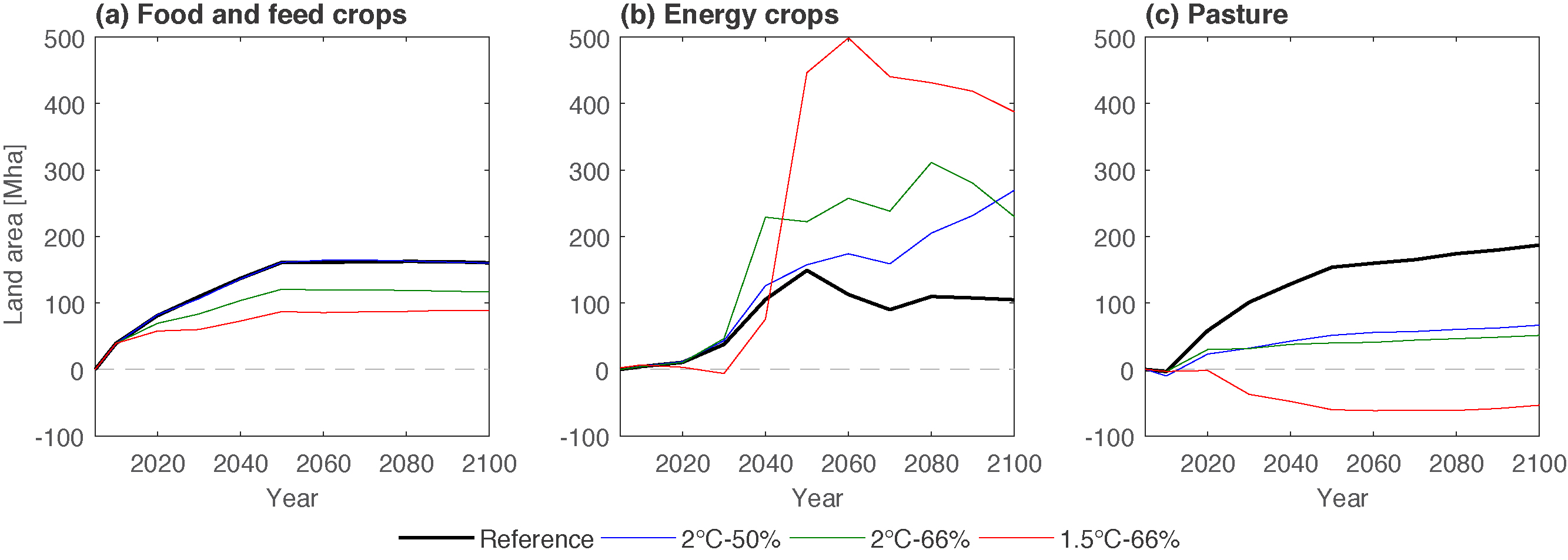
Figure 3. Refer to the following caption and surrounding text. — **Figure 3.** Change in global land for (a) food and feed crops, (b) energy crops and (c) pasture.
Download figure:
Standard image High-resolution image

Figure 4. Refer to the following caption and surrounding text. — **Figure 4.** Change in global land area for (a) forest and (b) other natural land (defined as land not used for agriculture purposes and not occupied by forest, such as natural grassland/steppe, savannah, tundra and desert).
Download figure:
Standard image High-resolution image

Land use

The increased demand for energy crops (figure 2(c)) translates to an increase in all scenarios of land used for energy crops (figure 3(b)) between 100 and 400 Mha by 2100 (peaking at 500 Mha in 2060 for 1.5 °C–66% scenario). This equates to 4% of global land area and, in the majority of regions, represents a change of <5% land area to energy crops but in some regions reaches 10%–15% (Ukraine, Rest of South Africa and South East Asia). There is an increase of ~325 Mha in one decade (2040–2050) in the 1.5 °C–66% scenario; for context this is over four times the global forest area loss in 1990s (Keenan et al 2015) and over four times the largest ten-year increase in herbaceous and woody crop land cover area in the period 1992–2015 (FAO 2018). One may argue that in reality more time will be needed to implement such an increase in bioenergy use. In all scenarios, there is a loss of other natural land (figure 4(b)), implying expansion of cultivation into these areas. Land for energy crop production is focussed in twelve regions that account for >96% of energy crop production in the three low emission scenarios (supplementary figures S3, S4 and S5). Within these regions, 33%–36% of production occurs in developed countries (figure S3), with 25 %–36% in Brazil, Russia and China (figure S4) and 33%–39% in other developing countries (figure S5). In the 1.5 °C–66% scenario after 2060 and 2 °C–66% scenario after 2080 there is an increase in bioenergy crop yields that enables an increase in energy crops (figure 2(c)) concurrent with a decrease in land area for energy crops (figure 3(b)).

Figures 3 and 4 are within the SSP scenario range (see figures 3 and 4 in Popp et al 2017), with notably a mid-range change in land for energy crops. SSP scenarios encompass a breadth of different trends. A key reason is that, at the moment, models show quite different trends for future global land use, reflecting different assumptions on yield development, barriers to trade, and land-use policies. The interplay between different land uses, and therefore trends in land use change over time, are highly complex and closely tied to future trends in population (demand), diet (how land is used), and agricultural practice (agricultural productivity and crop yields) (Powell and Lenton 2012, Slade et al 2014, Popp et al 2017). Estimates of future land availability for different functions differ greatly, often relating to different assumptions about land economics, food provision and nature conservation (i.e. avoiding deforestation to maintain carbon storage and biodiversity) (Slade et al 2014). Also, the use of local information on actual land use could lead to different land availability than estimated in global studies (Fritz et al 2013), while recently Daioglou et al (2017) showed that in several areas emissions from removing existing vegetation or foregone sequestration can be large and need to be accounted for.

To deliver negative emissions from BECCS it is essential that the bioenergy resource used is sustainable and has limited carbon emissions from direct and indirect land use change (Tilman et al 2009, Smith et al 2016, Daioglou et al 2017). In the scenarios, two thirds of energy crops are produced in China, Brazil, Russia and developing regions, potentially presenting a challenge for assurance of sustainable bioenergy production and limiting direct and indirect land use change emissions.

BECCS in the energy system

BECCS is net energy positive in contrast to other carbon dioxide removal methods, i.e. enhanced weathering, (Smith et al 2016). However, under certain deployment assumptions it may use more energy than it generates (Fajardy and Mac Dowell 2017).

Scenarios presented in the wider SSP narrative literature deploy a diversity of BECCS approaches, including BECCS within electricity, power, heating, liquid biofuel (potentially for aviation and shipping), hydrogen and biomethane pathways (see e.g. supplementary figure S15 in Bauer et al 2017). BECCS is principally used for electricity generation, hydrogen production and liquid biofuel production but the dominant technology differs greatly between SSP scenarios, for example over half the bioenergy used in SSP2-2.6 and SPP5-2.6 goes to liquid biofuels with CCS (Bauer et al 2017). The IMAGE model incorporates BECCS for power generation and hydrogen production, but not biofuel production. In the scenarios presented in this paper, BECCS is predominately used for electricity generation, with a small amount of hydrogen production after 2050 (figure S6).

Figure 5. Refer to the following caption and surrounding text. — **Figure 5.** Annual CO₂ stored by carbon capture and storage (CCS) and biomass energy with carbon capture and storage (BECCS) in Gt CO₂ per year. The three low emission scenarios are shown; no CCS occurs in the Reference scenario. The solid lines show total CCS and the dashed lines show the proportion of the CCS that is used for BECCS.
Download figure:
Standard image High-resolution image

Today, global road transport infrastructure is 'locked-in' to conventional combustion systems but it is currently predicted to shift towards electrification (Dominković et al 2017). Electricity generation by renewables such as wind and solar have been growing significantly in recent years (Jackson et al 2017). There are multiple possible uses of BECCS technologies and the potential future role for BECCS is strongly dependent on choices made across the energy system and the role of bioenergy within it.

Carbon capture and storage

CO₂ stored

In the scenarios generated by IMAGE, substantial levels of fossil CCS sit alongside BECCS in all scenarios (figure 5); total global cumulative storage (for fossil and biomass applications) is between 620 and 1295 Gt CO₂ in 2100 for the three low emission scenarios (table 2). CO₂ storage requires CCS infrastructure for both fossil and bioenergy CCS (see figure 1 and table 2), in power generation and industrial sectors, with fewer mitigation options for certain heavy industries, such as cement and steel. Furthermore, should direct air capture and storage be included in future scenarios, its geological storage requirements must also be included. Regional breakdown of the top ten CCS storage regions (supplementary table S3) shows that in 2100, global CCS activity is concentrated in five regions.

Global CO₂ storage capacity estimates vary hugely and are associated with considerable uncertainties (Bradshaw et al 2007, Koelbl et al 2013); similarly, at regional level, inherent differences between geological storage sites mean that each assessment will be different. Regional surveys are summarised in the Global Storage Portfolio (GSP) (GCCSI 2016a), although the approach, coverage and level of detail of these assessments vary (Consoli and Wildgust 2017). Similar to bioenergy resource potentials, geological storage can be categorised according to a resource pyramid describing theoretical, realistic or viable (Bradshaw et al 2007) or theoretical, effective, practical or matched capacity (CSLF 2007); in each case the uncertainty, costs and storage resource potential decrease with improved quality data. Table 2 presents the top five storage regions from the low emission scenarios compared to regional storage estimates taken from the GSP (Consoli and Wildgust 2017). Although the regional assessments presented are indicative, the magnitude of storage requirements in the scenarios sit within the range of available estimates (with the exception of Russia). In all three scenarios, the USA, China, India and Western Europe account for half of global storage. Storage requirements in China and USA require about 10% of the estimated capacity, while requirements in India and Western Europe are closer to the estimated capacities. The exception is Russia, where the modelled requirement for CO₂ storage exceeds the estimated regional storage capacity by an order of magnitude. By 2100, annual storage rates reach a maximum of 5.64 Gt CO₂ yr⁻¹ in the USA in the 1.5 °C scenario and are between 1.7–2.99 Gt CO₂ yr⁻¹ in the top four regions across all the low emission scenarios. Note also that the primary bioenergy regions in the scenarios are not the same as the primary CCS regions, with implications in high BECCS scenarios for both biomass energy trade and the 'common but differentiated responsibilities' principle (Peters and Geden 2017, UNFCCC 1992).

Table 2. Cumulative CO₂ emissions from carbon capture and storage (CCS), including BECCS in the top five storage regions in 2100. These five regions account for between 55% and 59% of global storage in each scenario. The regional data is compared to storage estimates based on relevant regional assessments (Consoli and Wildgust 2017). Assessment status relates to the quality of data used, e.g. 'Full' includes detailed national datasets, 'moderate' includes national studies without detailed resource calculations, 'limited' includes restricted studies based in selected sites, and 'very limited' is based on minimal or no data. Resource level relates to the level of detail of the assessment where 'theoretical' is at a regional/country scale, 'effective' at basin scale, 'practical' at a site scale, 'matched' is operational (Consoli 2016). Notes: (1) 'Best' estimate within the range low (500) to high (6000) (Hendriks et al 2004) as used in IMAGE model, note regional estimates cannot be aggregated to get a global capacity because of differences in methods and assumptions. (2) Global storage portfolio (GSP) data for Europe excluding UK, plus UK (both full, theoretical), plus Norway (full, effective).

Top five storage regions (in IMAGE)	Gt CO₂ (% of which is for BECCS)	Estimated regional resource Gt CO₂	Assessment status	Assessment detail (theoretical < effective < practical < matched)
1.5 °C–66% Scenario
Global	1295 (62%)	1660¹	—	—
USA	231 (60%)	2367−21 200	Full	Effective
China	179 (71%)	1573	Full	Effective
India	148 (78%)	47–143	Moderate	Theoretical
W Europe	107 (54%)	232²	Full	Theoretical/effective²
Mexico	93 (45%)	100	Moderate	Theoretical
2 °C–66% Scenario
Global	865 (43%)	1660¹	—	—
China	134 (55%)	1573	Full	Effective
USA	112 (48%)	2367–21 200	Full	Effective
W. Europe	93 (51%)	232²	Full	Theoretical/effective²
India	91 (40%)	47–143	Moderate	Theoretical
Russia	70 (85%)	6.8	Very limited	Theoretical
2 °C–50% Scenario
Global	618 (32%)	1660¹	—	—
China	94 (32%)	1573	Full	Effective
India	91 (36%)	47–143	Moderate	Theoretical
W. Europe	61 (40%)	232²	Full	Theoretical/effective²
USA	59 (25%)	2367–21 200	Full	Effective
Mexico	38 (10%)	100	Moderate	Theoretical

Nations with mature hydrocarbon industries will have industrial and institutional capacity and reservoirs are likely to be well characterised with proven trapping mechanisms and reliable seals. Delivery of CO₂ storage will require upfront investment in both infrastructure and the detailed site-specific appraisals of geological reservoirs (Sanchez and Kammen 2016). Onshore storage may be cheaper and, in engineering terms, more straightforward to use than offshore storage but may face considerable challenges in terms of public acceptability. As storage requirements accumulate, it is likely that costs will rise as more challenging sites are required (Bradshaw et al 2007). Delivery of CCS has proved challenging even in higher income nations with existing hydrocarbon industries and will prove more so for nations where such capacity is lacking (Sanchez and Kammen 2016). Storage is not the same as negative emissions (due to process and embedded emissions) and should not necessarily be used as shorthand for carbon dioxide removal levels (Gough et al in press).

Deployment rate

CCS is not used in the Reference scenario. Figure 5 shows the deployment of CCS and BECCS commence in the scenarios in 2020, with CCS increasing more quickly than BECCS by 2030. This reflects in part the lack of CCS infrastructure in 2017 and the climate policy action assumptions within these scenarios (i.e. delayed global climate policy action). The rate of deployment for CCS is at its fastest in the 1.5 °C–66% scenario in the 2030s, increasing from 1.72 GtCO₂ yr⁻¹ in 2030 to 11.16 GtCO₂ yr⁻¹ in 2040 (figure 5).

The key issues relating to deployment of BECCS represented in the scenarios are scale and speed of expansion. Introducing CCS technology adds a cost to existing power generation or industrial processes while at the same time rendering them less efficient. There are currently fewer than 20 CCS projects operational globally, capturing less than 40 Mt CO₂ per year. Of these, only one is a full chain power plant, one is a BECCS plant (GCCSI 2016b) and all are supported by government funding. Going from almost nothing to tens of Gt in the coming decades will require large capital investment in capture (including the engineering challenges of introducing biomass feedstocks (Finney et al in press)), transport and storage infrastructure. This presents a bottleneck in terms of both financing and construction, with significant economic and regulatory challenges (Herzog 2011, Bhave et al 2017). Assumed deployment rates are challenging; although some analysis suggests these fall within historical rates of capacity addition for other energy technologies (van Sluisveld et al 2015) others suggest it may exceed those seen previously in fossil technologies (McGlashan et al 2012) or renewable and nuclear (Torvanger et al 2013). It is clear that the deployment of BECCS will require ambitious policy interventions (Peters and Geden 2017).

Figure 6. Refer to the following caption and surrounding text. — **Figure 6.** Comparison of the way a generalised BECCS system is represented in the IMAGE model versus a Life Cycle Analysis approach. Left column depicts the stages in a generalised BECCS system as it may be analysed in a LCA (stages 1–8) (modified from Thornley *et al* (2015) and Smith and Torn (2013)). Middle column depicts a generalised BECCS system as represented within the IMAGE model (stages (a)–(d); green shading represents processes within the land use model and blue shading the energy system model (Stehfest *et al* 2014). Right column identifies where emissions are reported in IMAGE model output (i-v). Note AFOLU means agriculture, forestry and other land use.
Download figure:
Standard image High-resolution image

Social acceptability

While social acceptability is not explicitly represented in the models, it is crucial and potentially unpredictable in the context of rapid expansion of a new technology on a very large scale. Several planned CCS projects, notably in northern Europe, have failed after facing significant public opposition. Two key factors affecting public responses are scale, with smaller scale operations more likely to be accepted, and early involvement in planning and consultation (e.g. Dütschke 2011); a rapid, massive expansion in large scale projects may challenge public responses on both fronts. While offshore storage projects have typically received a less hostile reception than onshore projects, research suggests that this cannot necessarily be taken for granted (Haug and Stigson 2016, Mabon et al 2014). The small number of operational CCS projects to date may not be a reliable indication of how a rapid rollout might proceed. It is similarly difficult to generalise about the future social response to potentially large-scale changes in bioenergy production, given the heterogeneity of feedstocks, their sources and affected local communities. Some insights can be gained from sustainability assessments (economic, environmental and social) at a local scale of present day large scale forest plantations in Chile and Spain (e.g. Andersson et al 2015, Diaz-Balteiro et al 2016).

Representing negative emissions delivered by BECCS

The delivery of negative emissions, i.e. removal of carbon from the atmosphere, by BECCS is a result of capturing (during the energy conversion process) and storing (in geological reservoirs) CO₂ taken up from the atmosphere by biomass during its growth (Kemper 2015). There are process emissions at all stages in a BECCS system, through direct CO₂ emissions from the energy used during cultivation, harvest, processing and transport, emissions of methane or nitrous oxide (e.g. during drying (Röder and Thornley 2016) or fertiliser use) and direct carbon loss from soils due to changes in land use (e.g. conversion from grassland to bioenergy crop). The amount of CO₂ stored underground does not equate directly to carbon removed from the atmosphere, due to these process and land use emissions (Gough et al in press). In figure 6, we present a comparison of how the stages of a generalised BECCS system are presented within the IMAGE model and from a life cycle analysis perspective (Thornley et al 2015, Smith and Torn 2013). Although LCA and IAM are different approaches with different functions, this highlights some of the details considered in an LCA (figure 6, left column) that are not included within an IAM (figure 6, middle column), such as drying and chipping.

Most scenarios now emphasize the potentially significant role of removing carbon dioxide from the atmosphere in achieving the aspirations of the Paris Agreement (Fuss et al 2014, Clarke et al 2014, van Vuuren et al 2013). A number of studies have raised concerns over how negative emissions from BECCS systems are calculated (Fajardy and Mac Dowell 2017, Vaughan and Gough 2016, Gough et al in press). Within IMAGE, the emissions associated with land use change (figure 6 (i) and from fertiliser (figure 6 (ii)) are accounted for under agriculture, forestry and other land use (AFOLU) emissions. The process emissions are accounted for within the energy system (figure 6 (iii) and (iv)) and the contribution to emission reductions from BECCS represents CO₂ stored (figure 6 (v)). This means that, although IMAGE (particularly due to its spatially explicit land use model) captures all the key process and land use change emissions, these are usually not presented as a single value reporting the net carbon removed by BECCS. Factors that are not captured currently within IMAGE include the impact of albedo changes and climate feedbacks due to land use change (Smith et al 2016).

In summary, there are seven main assumptions in IMAGE that lead to the large-scale use of BECCS:

1.
Cost-optimisation and the use of some discounting.
2.
Strong regulation and governance of bioenergy production (i.e. the protection of forest and food production land).
3.
Mid-range assumptions about the availability of CO₂ storage capacity combined with optimistic assumptions about CCS infrastructure development.
4.
Development of a well-functioning large-scale biomass energy market (i.e. provide residues to large-scale power plants).
5.
Technology development in energy crops, energy conversion technologies and capture technologies.
6.
Early investment into CCS/BECCS allowing technological learning.
7.
Assumptions about the limits of contributions from other technologies (e.g. renewables).

Conclusions

Emissions reductions necessary to achieve the aspirations of the Paris Agreement (UNFCCC 2015) may be unachievable without large-scale use of BECCS (Larkin et al 2017, Fuss et al 2014). BECCS could occupy a variety of roles within the energy system, dependent upon both technological advances (e.g. hydrogen production) and overall energy system decarbonisation trends (e.g. electrification of road transport). Biomass residues are an important biomass resource accounting for about half of the bioenergy in the IMAGE scenarios presented here; they are associated with fewer sustainability concerns than dedicated bioenergy crops (e.g. Tilman et al 2009). In the IMAGE model runs presented here it is assumed that policies prevent dedicated bioenergy crops to be grown on forest land or land used for food production. However, ensuring that this is the case in reality depends upon the robustness of regulatory frameworks at a regional level; in the scenarios presented, only a third of bioenergy crops are assumed to be grown in developed countries with established regulatory frameworks. A failure to assure that bioenergy crops are grown on land with minimal carbon loss from direct and indirect land use change can significantly impact the amount of carbon removed from the atmosphere by BECCS (Daioglou et al 2017, Fajardy and Mac Dowell 2017).

Global CO₂ storage capacity estimates are of limited use due to the regional variation of storage opportunities, variation in assessment methodologies and data availability. Here we present a regional breakdown of storage requirements in IMAGE and compare these to recent regional estimates (and their associated data quality). In the IMAGE scenarios half of all global storage required by 2100 occurs in USA, Western Europe, China and India, all are within the range of their respective regional storage resource estimates. Deployment rates for CCS in the scenarios are challenging and may exceed those seen previously in fossil, renewable or nuclear technologies and will require ambitious policy interventions. It is important to note that without climate policy action (i.e. in the Reference scenario) there is no CCS. Societal responses to BECCS will vary regionally and over time, and may constrain deployment rates. Evidence suggests that potential issues are most likely to arise with onshore storage sites and some forms of large-scale bioenergy crops.

The IMAGE model captures the key process and land use change emissions that can influence the net CO₂ removed by a BECCS system, but this is not explicitly quantified in a single value. For example, land use change emissions arising from the bioenergy crops used to supply a BECCS system are reported under agriculture, forestry and other land use (AFOLU) emissions. Therefore, while all the relevant emissions are included in the estimates of global net emissions in relation to carbon budgets within the model, taking the figures for negative emissions (e.g. figures 1 and 5) in isolation may be misleading.

Overall, the scenario outcomes in the IMAGE model are ambitious but consistent with current relevant literature for specific assumptions. Key assumptions about the bioenergy and CCS necessary for BECCS fall within the mid-range of other scenarios and other literature data, although there remains limited empirical data available. The results from the IMAGE model are consistent across the scenarios analysed in this paper. IMAGE, and other IAMs with spatially explicit land use, are extremely useful tools to explore possible options and impacts of BECCS. Their value as heuristic tools, however, does not replace the need for detailed and specific analyses of the underlying concepts, assumptions and scenario outcomes to understand better the implications and consequences of ambitious climate policy goals.

Acknowledgments

This paper was funded by the UK Government, Department for Business, Energy and Industrial Strategy, as part of the Implications of global warming of 1.5 °C and 2 °C project. NEV, CG & EWL acknowledge support from the Natural Environment Research Council (NE/P019951/1). NEV thanks BGM Webber and C Le Quéré for input and discussions.

Dates

Peer review information