

Abstract
Urban vegetation provides many highly valued ecosystem services but also requires extensive urban water resources. Increasingly, cities are experiencing water limitations and managing outdoor urban water use is an important concern. Quantifying the water lost via evapotranspiration (ET) is critical for urban water management and conservation, especially in arid or semi-arid regions. In this study, we deployed a mobile energy balance platform to measure evaporative fraction throughout Riverside, California, a warm, semi-arid, city. We observed the relationship between evaporative fraction and satellite derived vegetation index across 29 sites, which was then used to map whole-city ET for a representative mid-summer period. Resulting ET distributions were strongly associated with both neighborhood population density and income. By comparing 2014 and 2015 summer-period water uses, our results show 7.8% reductions in evapotranspiration, which were also correlated with neighborhood demographic characteristics. Our findings suggest a mobile energy balance measurement platform coupled with satellite imagery could serve as an effective tool in assessing the outdoor water use at neighborhood to whole city scales.
Export citation and abstract BibTeX RIS
1. Introduction
Urban vegetation provides a wealth of ecosystem services to local residents including cooling, foods, and aesthetic appeal with many connections to immediate health concerns and improved well-being (Pataki et al 2013, Jenerette et al 2011, Fuller et al 2007, Alaimo et al 2008). In light of the benefits, policy goals for many cities are to expand urban vegetation density, primarily as trees (Pincetl 2010). However, the water requirements for providing vegetation-based ecosystem services can be large and pose a fundamental tradeoff for their use in water-limited environments (Jenerette et al 2011, Pataki et al 2011a). Uncertainties in outdoor water use restrict the abilities of models to quantify or forecast urban water demands, hydrologic dynamics, and the effect of policies for managing water resources (Bhaskar et al 2015, Vahmani and Hogue 2014, Shaffer et al 2015, Pataki et al 2011a). With increasing droughts and competition for water among urban, agricultural, and in-stream uses, considering the water requirements embodied within ecosystem services is essential.
In semi-arid and arid environments outdoor urban water use can be large and intense, potentially exceeding 50% of total water use at the household scale (Mini et al 2014) and with evapotranspiration (ET) rates that can approach reference ET (Litvak et al 2017a). High variability in outdoor urban water use is also expected and may exceed an order of magnitude difference among neighborhoods (Jenerette et al 2011). Nevertheless, few direct estimates of outdoor water magnitude are available. Individual agency reporting of water deliveries are typically used for verification of urban water use (Mini et al 2015). Reported data are frequently an aggregate measure that removes spatial variation and has sources of uncertainty such as leakage from aging pipes. However, self-reported 'bottom-up' data do not provide information specific to outdoor versus indoor water use but require an assumed fraction of total water deliveries that is not well characterized. Direct measurements of ET, the water flux most connected to outdoor water use, have been obtained from small plots using chamber measurements and from individual trees using sap flux measurements (Bijoor et al 2014, Litvak et al 2017b). Scaling these measurements to parcel, neighborhood, or whole cities remains a key research challenge. Alternatively, fixed towers using eddy covariance based micrometeorological approaches have measured outdoor water fluxes at individual neighborhood scales (Grimmond and Christen 2012). Limited work conducted in hot, arid regions has suggested relatively low ET fluxes, although these may better reflect specific site characteristics rather than whole city distributions (Roth 2007, Chow et al 2014). Direct estimates of outdoor urban water flux that resolve variation within neighborhoods and across whole cities are needed to better understand urban ecohydrology and allow improved management of water resources and ecosystem services.
One prominent management policy implemented in response to droughts is water restrictions (Kenney et al 2008, Maggioni 2015, Milman and Polsky 2016). As a recent example, in 2015 following a historically unprecedented drought in California, a gubernatorial executive order mandated an average 25% reduction in water use by all urban water supply agencies (Reese et al 2015). A primary focus of this restriction was outdoor water use associated with irrigation practices (Boxall et al 2015). However, the effectiveness of water restriction mandates and conservation programs at reducing actual outdoor water use is difficult for water managers to assess on an individual parcel to neighborhood scale (Mini et al 2015). Evaluations of water restrictions on water use have suggested mixed effectiveness (Mini et al 2015). An empirical evaporation based assessment of water restriction effectiveness on reducing outdoor water use and its spatial distributions would provide independent evaluation of water use, its sensitivity to restrictions, and sources of variation within a city.
Urban demographic characteristics at neighborhood scales can have a large influence on the spatial distribution of both vegetation and likely outdoor water use (Jenerette et al 2013, Jenerette et al 2016). Given the positive correlation between vegetation and neighborhood socioeconomic status, higher neighborhood incomes have also been connected to greater water uses and increasing water uses during hotter and drier periods (Syme et al 2004, Balling et al 2008, Ouyang et al 2016). In response to water restrictions, data from water deliveries also suggested both increased lot size and income were associated with greater reductions in water use and supported a hypothesis that water reductions are related to opportunities to reduce water conservation (Mini et al 2015, Renwick and Archibald 1998). While income–outdoor water use relationships and sensitivity to water restrictions have been hypothesized, tests of these relationships with direct measurements of outdoor water use are still needed.
In this study, we use a mobile micrometeorological platform to measure regional ET at numerous locations across an urbanized landscape in Riverside, California (CA), USA. Riverside is an inland city representative of recent urbanization in southern California away from cooler summer coastal conditions (Tayyebi and Jenerette 2016). We evaluated relationships between in-situ energy balance measurements and remote sensing-based vegetation greenness indices using the regional evaporative fraction energy balance (REFEB) approach (Anderson and Goulden 2009). With the resulting models, we mapped the spatial variation in ET for August in 2014 and 2015, prior to and following mandatory 25% water restrictions, across urban land covers and neighborhoods that differed in vegetation density. We examined spatial variation in water reductions and evaluated relationships between outdoor water use and demographic variation among neighborhoods. Through these analyses, we provide the first spatially distributed measurements of urban ET, generate a tool for rapid mapping of ET distributions, test the effectiveness of water restrictions on reducing ET, and evaluate how water use and associated policy interventions are linked to demographic characteristics.
2. Methods
2.1. Experimental design and data collection
The study area is in the city of Riverside, located in semi-arid southern California, USA (figure 1). This region is characterized by a Mediterranean climate of alternating cool-wet winters and hot-dry summers with little to no rain. Annual rainfall is ∼280 mm, with 2014 and 2015 having less than 220 mm year−1 during the drought (see supplementary table S1 available at stacks.iop.org/ERL/12/084007/mmedia). Irrigated, urban vegetation in the study area provides substantial summertime cooling (Shiflett et al 2017). The domestic water usage in Riverside mainly relies on imported water or senior groundwater rights to nearby basins. Summer flow of the Santa Ana River, a significant riparian area on the north side of the city, primarily originates from effluent discharges of upstream municipal wastewater treatment facilities such as the Rapid Infiltration and Extraction facility, the Rialto Wastewater Treatment Plant. Average summer stream flow of the Santa Ana River is about 1.17 m3 s−1, which is reduced approximately 34% relative to the average winter stream flow of 1.78 m3 s−1 (table S1).
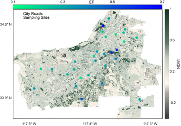
Figure 1 Spot evaporative fraction (EF) measurements (n = 29) across Riverside, CA on a base map composed of NDVI and city roads (www.dot.ca.gov/hq/tsip/gis/datalibrary/). The color of each point location presents the mean measured EF value from EC.
Download figure:
Standard image High-resolution imageIn total, 29 locations were selected using three criteria: (1) site accessibility, including public and road access for the mobile platform; (2) coverage of the main landscapes, including neighborhoods (NB) with low or high vegetation density, industrial/commercial district (ICD) and public green spaces (e.g. parks and golf courses) or agricultural area (GSA) and (3) relatively uniform distribution of the sites. A mobile tower attached to a trailer was moved to sampling sites around the city in order to collect observations. An open-path infrared gas analyzer (IRGA) (LI7500, LI-COR, Lincoln, Nebraska, USA) was installed with a three dimensional sonic anemometer (CSAT3, Campbell Scientific, Logan, Utah, USA) on the tower to record water vapor concentration, wind speed, and virtual air temperature at 10 Hz. Other meteorological sensors, including temperature and relative humidity probes (HMP45C, Vaisala, Helsinki, Finland) and a four-component net radiometer (NR01, Hukseflux Delft, Netherlands), were also mounted on the tower. The tower, while temporarily parked at each site, was extended up to 12 meters high to obtain an adequate flux footprint depending upon vegetation height. We collected data for approximately one hour; IRGA and sonic anemometer measurements were separated into 10-minute intervals for the EF calculation; other meteorological measurements were collected every 10 minutes concurrently. Under clear sky conditions, daily sampling was conducted between 10:30 to 16:30 Pacific Daylight Time (PDT) to minimize daily variation of evaporative fraction (EF) (Shuttleworth and Wallace 1985, Anderson and Goulden 2009). The sampling period occurred from July 28th to August 28th, 2015.
2.2. EF calculation from micrometeorological measurements
EF, defined as the ratio of latent heat to available surface energy, uses an inherent connection between ET and available surface energy to map the regional distribution of ET (Anderson and Goulden 2009, Anderson et al 2012). EF was measured using the REFEB approach (Anderson and Goulden 2009). REFEB relies on using high frequency temperature (T) and specific humidity (q) observations to calculate the Bowen ratio (B) at a single height using the regression method of DeBruin et al (1999) as shown in equation 1:
where γ is the psychrometric constant and T' and q' are the fluctuations of T and q determined from Reynolds averaging. EF can be obtained from B as shown in equation 2:
In practice, the one hour measurement interval from each site was separated into 10-minute intervals, which follows the regression period length used by Anderson and Goulden (2009). For each period, a regression between the variance of temperature (T') and specific humidity (q') was conducted to retrieve the slope and calculate B and EF. Also following Anderson and Goulden (2009), we used the correlation between T and q (rTq) as a data quality indicator and discarded data points with rTq less than 0.25.
2.3. Calculation of ET
Along with the mobile tower, we installed two eddy covariance (EC) stations, one in an industrial district and another at an agricultural orchard site, as low and high end-points in vegetation coverage to monitor the diurnal pattern of EF and to test self-preservation of EF. Based on the two-endpoints of EC measurements, variation of EF at low-vegetation sites was less than 10% compared to the midday measured EF (figure S1). As Lhomme and Elguero (1999) pointed out, good EF measurements can be obtained 'in the central hours of the day, and preferably about three hours before or after noon' under clear sky conditions. Here, we chose a time window spanning from 10:30 to 16:30 PDT based on vegetation cover at each site to maximize the measurements of EF in a single day. Then we averaged the calculated EF within about an hour (four to seven individual EF measurements) to represent the EF at each site. This has shown to be effective for other regional ET studies where low diurnal variation in EF did not affect regional ET calculations (Anderson and Goulden 2009, Isaac et al 2004).
We retrieved an empirical model between measured EF and normalized differential vegetation index (NDVI) using ordinary least squares linear regression. The NDVI map was calculated from the surface reflectance product (C1 higher-level) of Landsat 8 OLI/TIRS images (Band 4 and Band 5) downloaded via the US Geological Survey Earth Explorer (http://earthexplorer.usgs.gov). The surface reflectance product was atmospherically corrected to allow interannual comparison of NDVI and the estimates of ET. Since NDVI could decline with drought (Tadesse et al 2014, Vicente-Serrano et al 2013) during our sampling period (July 28th to August 28th), we used the available surface reflectance products (July 31st, August 16th and September 1st) acquired from July 31st to September 1st 2015 and linearly interpolated the calculated NDVI across the sampling period to match the collected EF at each sampling date. A 50 m buffer was generated around the coordinates of each site. Then we extracted NDVI values within each buffer and used the mean NDVI to represent vegetation greenness at each site. After matching the calculated NDVI and measured EF at each site and date, we further applied a 1000-iteration bootstrapping to regress the NDVI and EF to obtain more robust parameter estimates. Based on the empirical relationship between measured EF and calculated NDVI, we implemented this model to obtain the spatial EF distribution in Riverside.
Finally, EF was extrapolated to calculate the latent heat (LE) fluxes following the energy balance equation:

where the A denotes the available energy, Rn is the net radiation and G is the ground heat flux (all in units of W m−2). At daily to monthly scale, we expect G was negligible (Cleugh et al 2007, Mu et al 2007). The Rn is obtained from NASA's Clouds and the Earth's Radiant Energy System (CERES) monthly average total flux surface product (EBAF–surface). Anderson and Goulden (2009) have shown that CERES combined with NDVI driven EF was able to observe monthly ET with minimal discrepancy. We chose the all sky solar radiation in August 2015 (188.65 W m−2) as a surrogate to calculate the latent heat flux from equation (3) since the all sky net radiation covers all the periods for each month and provides better ET estimates at monthly scale (Wielicki et al 1996). The latent heat flux (LE, W m−2) was converted to evaporation (ET, mm day−1) using the latent heat of vaporization at 20 °C (2.45 MJ kg−1). Applying the same relationship between EF and NDVI, we also quantified the ET difference between August 2014 and 2015, and further explored inter-annual effects of dynamic vegetation greenness on ET variation, via the NDVI from Landsat 8 OLI/TIRS images (August 13th) and the Rn in August of 2014 (198.94 W m−2) under the all sky condition from CERES.
To investigate potential socioeconomic correlations with ET, we retrieved the population and annual income per capita across 204 city blocks in Riverside from the 2010 United States Census using the Census Bureau's Factfinder website (http://factfinder.census.gov). The modelled ET and the ET difference between 2014 and 2015 were averaged by block, and a simple linear regression model between ET or ET difference and population or income was applied.
3. Results
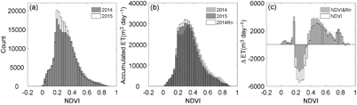
A substantially higher daytime EF value (0.69 ± 0.09, mean ± SD) was consistently observed at the vegetation dominated, irrigated orchard EC tower compared to the impervious surface dominated industrial tower (0.36 ± 0.05) (figure S1). These continuous measurements at the two land cover endpoints showed consistent meteorological conditions during all of our distributed measurements. At the 29 discrete sampling locations from ICD, NB and GSA land, we obtained a total of 185 valid EF measurements with 10-minute measured intervals. EF was significantly higher in the more vegetated GSA rather than in the less vegetated ICD and NB (p < 0.0001 ANOVA; figure 2(a)). Among these sites we found a strong relationship between EF and satellite-derived NDVI in our study (R2 = 0.71 ± 0.11, p < 0.0001, figure 2(b)). The NDVI derived from the 50 m buffer ranged from 0.10 to 0.71 but had a higher variability in NB (0.33 ± 0.10) and GSA (0.57 ± 0.11) than ICD (0.15 ± 0.06) land covers. Based on the empirical regression model, NDVI explained 71% ± 11% of the EF variation in our study region (figure 2(b)). This further suggests ET increased by about 1.1 mm day−1 with the increase in greenness (NDVI) from ICD (0.15) to GSA (0.57) under a net radiation of 100 W m−2.
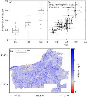
Figure 2 The relationship between EF and greenness (NDVI) and the estimated difference of ET between August 2015 and 2014. (a) Presents an ANOVA comparison of EF among different landscape types, i.e. industrial or commercial district (ICD), neighborhood (NB) and green space (GS). (b) Shows the regression analysis between measured EF and satellite-based NDVI, and (c) depicts the modelled ET difference (∆ET) between 2014 and 2015 based on the regression model from (b).
Download figure:
Standard image High-resolution imageUsing the relationship between EF and NDVI and CERES net radiation, we developed ET maps across Riverside for August 2015 (figure S2) and 2014. These maps show high mean ET (3.77 ± 0.20 mm day−1) over golf courses (3.77 ± 0.20 mm day−1) and agricultural regions (2.99 ± 0.44 mm day−1) at 2015. As expected, relatively low ET was found in areas with limited vegetated or primarily impermeable surface. The average ET difference between 2014 and 2015 is 0.16 ± 0.23 mm day−1, with an average 7.8% decrease in 2015 compared to 2014 (figure 2(c)). Well-vegetated regions (NDVI above 0.6) had the largest absolute reductions, with reduced ET of 0.29 ± 0.27 mm day−1, which is about 75% higher than the average ET reduction.
We found clear patterns among ET, population density, and socioeconomic status. ET was negatively correlated to population density across 204 blocks in Riverside but was positively correlated to the annual income per capita at each block (figure 3). This is consistent with Riverside's most expensive housing being co-located with golf courses and the agricultural greenbelt in the western part of the city. Furthermore, the ET difference between 2014 and 2015 shows a similar pattern (figure 4), demonstrating the change in ET between 2014 and 2015 ([2014–2015]/2014 × 100%) from blocks with lower population is larger than the blocks with high population, but there is no significant correlation between ET difference and annual income per capita.

Figure 3 Relationships between estimated mean ET and socioeconomic census data from 204 city blocks in Riverside. (a) Demonstrates the trend between ET and population using a linear function as y = ax + b. The slopes are statistically significant different (p = 0.0002) between 2014 and 2015, while (b) shows how ET responds to increasing income per capita. Circles represent data from 2014 and black dots refer to 2015 data. The dashed line refers to the regression from 2014 data and the solid one refers to 2015.
Download figure:
Standard image High-resolution image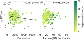
Figure 4 Relationship between estimated mean ET difference as percentage (∆ET(%), [2014–2015]/2014 × 100%) and socioeconomic census data at the block scale in Riverside. (a) Demonstrates the trend between ∆ET and population fitting by a linear relationship as y = ax + b, and (b) shows the response of ∆ET to increasing income per capita. The colour gradient represents the average vegetation cover (percentage, %) at each block.
Download figure:
Standard image High-resolution image4. Discussion
We quantified the relationship between field EF measurements and satellite-based vegetation indices in Riverside, CA thereby providing the first empirical estimates of the spatial distribution of outdoor urban water use. Compared to water provider data that supplies a bottom-up and spatially aggregated estimate of total water use, our analyses provide a top-down and spatially distributed estimate of outdoor water use. Our approach combines in-situ measurements of whole ecosystem water fluxes with satellite based vegetation greenness indices. In non-urban environments vegetation indices can predict up to 70% of EF variation (Wang et al 2006, Anderson and Goulden 2009) and here we show similar predictive skill in the highly heterogeneous urban environment. On average, the summer rainfall in Riverside during the dry season (June, July and August) is only 0.25 mm day−1 (table S1), which contributes about 13% of the ET of Riverside, with an average ET of 1.8 mm day−1 from the prediction using REFEB approach. The remaining 87% of ET is directly from municipal water use-derived riparian ET (Townsend-Small et al 2013). The REFEB approach can provide valuable information for modeling urban water use and evaluating the effectiveness of policies for water reductions.
The spatial distribution of water use in Riverside, CA was consistent with hypotheses for the influences of population density and socioeconomic distributions. Higher population density neighborhoods had lower ET reflective of more developed areas and less green space for irrigation. Higher income regions used extensively more water, reflective of a luxury effect (Hope et al 2003, Jenerette et al 2011), and higher greenness is considered a desirable housing aspect which can command higher prices (Astell-Burt et al 2014). This luxury effect in water use is consistent with previous assessment from Los Angeles, CA using water delivery data (Mini et al 2015). Conversely, less greenness is associated with higher levels of multifamily housing, which is linked to both higher population density and lower income levels. We found clear relationships between ET and socioeconomic factors, i.e. population and annual income (figure 3). The interannual ET difference is also significantly correlated with population at the block scale (figure 4(a)). Recognition of socioeconomic effects on urban vegetation distribution has increasingly become an environmental justice concern (Wolch et al 2014) and we also show here important consequences for water distributions, although these relationships are need further evaluation across a range of arid and semi-arid regions.
During August between 2014 and 2015 we observed a 7.8% reduction in ET across the entire city. Our observation falls within the reported reduction in total water use by the city of Riverside of 12.5% between August 2014 and 2015 (California State Water Resources Control Board). This difference suggests outdoor water reductions shared a considerable proportion of total reductions. In part the outdoor water use reductions associated with water restrictions were related to socioeconomic variation among neighborhoods with the greatest absolute reductions occurring in high income neighborhoods. Nevertheless, the distribution of water reductions was proportional with pre-restriction use and also consistent with population density and socioeconomic patterns. However, the interannual variation of net radiation could also result in interannual difference in ET estimates and such data from satellite data have potentially substantial uncertainties. Compared to 2014, the net radiation from CERES observations in 2015 decreased ∼5% from 198.9–188.7 W m−2. To estimate the percentage of change in CERES Rn that could be due to water restrictions we compared incoming solar irradiance from spatial CIMIS (Hart et al 2009) for downtown Riverside and MODIS albedo and skin temperature for the extent of Riverside using the Oak Ridge National Laboratory subset tool (ORNL DAAC 2008a, ORNL DAAC 2008b). Incoming solar irradiance actually increased from 2014 to 2015 (293.8–297.3 W m−2) slightly while albedo and surface temperature also increased minimally, 0.0015 and 0.019 K respectively. In contrast, urban vegetation decreased, consistent with a landscape effect of the urban water restriction mandate in year 2015. Potential interactions between Rn and vegetation also result from changes in surface reflectance that could result in lower net radiation with browning vegetation. Vegetation independent estimates of net radiation that can more appropriately quantify urban energy balance variation remain an important research need in estimating regional ET using the REFEB approach.
To better identify the interactions between changes in vegetation and net radiation we explored their interactive influence on regional ET variation. NDVI difference between 2014 and 2015 showed a clear land surface change across the two years (figure 5(a)), with a lower NDVI in 2015 at vegetated regions (NDVI > 0.4) or impermeable surfaces (NDVI < 0.1) and a higher NDVI at limited vegetated regions or bare soils (NDVI between 0.1 and 0.4). We compared the ET change across varying vegetation levels in 2014 and 2015 and found a clear decrease of ET within more densely vegetated regions (figure 5(b)). To evaluate the effects from the interannual Rn variation on ET, we used the same Rn as 2014, i.e. 198.9 W m−2, to calculate the ET in 2015. This analysis provided an indication of the magnitude of ET reduction due to vegetation changes alone (figure 5(b)). At the whole-city scale, in vegetated regions (NDVI > 0.4) changes in NDVI contributes 83.3% of the ET difference between 2014 and 2015 (∆ET = 2014–2015) on average, with a mean ∆ET of 2313.6 m3 day−1 by including Rn and NDVI effects, but a mean ∆ET of 1442.4 m3 day−1 by only accounting for NDVI (figure 5(c)) using the same Rn in the two years. Hence, at least 6.5% of ET reduction in vegetated regions accounted for the average 7.8% reduction in ET across the whole city.
Figure 5 The NDVI and ET difference between 2014 and 2015. (a) Shows the NDVI in well-vegetated regions (NDVI > 0.4) decreased in 2015 (clear bars) compared to 2014 (grey bars). (b) Demonstrates the ET estimates in 2014 (grey bars) and 2015 (dark bars) by using the CERES Rn estimates in 2014 and 2015, respectively. The clear bars show the ET estimates in 2015 using the Rn estimates in 2014 to excluding the effects from Rn difference. (c) Shows the ET difference (2014–2015). The grey bars show the ET difference by including the NDVI and Rn effects on ET estimates. The clear bars only demonstrate the NDVI effects on ET estimates by applying the same Rn value as 2014 to calculate the ET in 2015.
Download figure:
Standard image High-resolution image
Vegetation is a key component of cities throughout the world (Forman and Wu 2016). The ecosystem services derived from vegetation within a city are directly connected to human well-being through multiple ecosystem services. However, the provisioning of ecosystem services within a city has a key tradeoff in the associated need for water (Jenerette et al 2011, Pataki et al 2011a). In cities located in arid or semi-arid areas, like Riverside in semi-arid southern California, evaluating the water use associated with vegetation is a key research need. For example, a recent state regulation in California that reduces turf grass area to a maximum of 25% of landscaped area in new developments (Reese et al 2015) may have a long-term impact on water savings accordingly. Our findings reflect differences in peak summer ET among the different sites and provide support for the role of mandated water restrictions to reduce outdoor water usages. Nevertheless, reducing the percentage of vegetation cover also has consequences for reduced availability of ecosystem services and potential feedbacks to water use. A recent study suggested that increasing vegetation cover could decrease the urban heat island and also decrease plant water requirements in urban regions (Zipper et al 2017). In addition to the amount of vegetation coverage, species differences can also influence water use (Pataki et al 2011b) and better species information may help refine outdoor water use estimates. Managing urban water use and ecosystem services require new data sources that can readily estimate spatial and temporal dynamics of urban water use. Our results show how a mobile energy balance measurement platform can be coupled with satellite greenness to obtain empirical maps of outdoor water use and assess the effectiveness of outdoor water interventions at the whole city scale.
Acknowledgments
We thank Lindy Allsman and Dennise Jenkins for their assistance with the eddy covariance towers and mobile observations. We also appreciate Steven Crum, Peter Ibsen, Holly Andrew and Mia Rochford for help with the field EC measurements, Amin Tayyebi for helping with GIS analysis, and Kurt Schwabe for valuable insights on local water policy and data. This research was supported by National Aeronautics and Space Administration (NASA) through grant NNX12AQ02G, NNX15AF36G and the National Science Foundation (NSF) through grant DEB-0919006, and the UWIN Sustainability Research Network and by USDA-ARS National Program 211: Water Availability and Water Management (project number 2036-61000-015-00). Field micrometeorological data used in this study are available by contacting L L Liang or G D Jenerette at lssllyin@gmail.com or darrel.jenerette@ucr.edu, respectively.
Footnotes
5 The US Department of Agriculture (USDA) prohibits discrimination in all its programs and activities on the basis of race, color, national origin, age, disability, and where applicable, sex, marital status, familial status, parental status, religion, sexual orientation, genetic information, political beliefs, reprisal, or because all or part of an individual's income is derived from any public assistance program. (Not all prohibited bases apply to all programs.) Persons with disabilities who require alternative means for communication of program information (Braille, large print, audiotape, etc.) should contact USDA's TARGET Center at (202) 720–2600 (voice and TDD). To file a complaint of discrimination, write to USDA, Director, Office of Civil Rights, 1400 Independence Avenue, S.W., Washington, DC 20250-9410, or call (800) 795–3272 (voice) or (202) 720–6382 (TDD). USDA is an equal opportunity provider and employer.
Mention of trade names or commercial products in this publication is solely for the purpose of providing specific information and does not imply recommendation or endorsement by the US Department of Agriculture.