

Abstract
The Corn Belt states are the largest corn-production areas in the United States because of their fertile land and ideal climate. This attribute is particularly important as the region also plays a key role in the production of bioenergy feedstock. This study focuses on potential change in streamflow, sediment, nitrogen, and phosphorus due to climate change and land management practices in the South Fork Iowa River (SFIR) watershed, Iowa. The watershed is covered primarily with annual crops (corn and soybeans). With cropland conversion to switchgrass, stover harvest, and implementation of best management practices (BMPs) (such as establishing riparian buffers and applying cover crops), significant reductions in nutrients were observed in the SFIR watershed under historical climate and future climate scenarios. Under a historical climate scenario, suspended sediment (SS), total nitrogen (N), and phosphorus (P) at the outlet point of the SFIR watershed could decrease by up to 56.7%, 32.0%, and 16.5%, respectively, compared with current land use when a portion of the cropland is converted to switchgrass and a cover crop is in place. Climate change could cause increases of 9.7% in SS, 4.1% in N, and 7.2% in P compared to current land use. Under future climate scenarios, nutrients including SS, N, and P were reduced through land management and practices and BMPs by up to 54.0% (SS), 30.4% (N), and 7.1% (P). Water footprint analysis further revealed changes in green water that are highly dependent on land management scenarios. The study highlights the versatile approaches in landscape management that are available to address climate change adaptation and acknowledged the complex nature of different perspectives in water sustainability. Further study involving implementing landscape design and management by using long-term monitoring data from field to watershed is necessary to verify the findings and move toward watershed-specific regional programs for climate adaptation.
Export citation and abstract BibTeX RIS

Original content from this work may be used under the terms of the Creative Commons Attribution 3.0 licence.
Any further distribution of this work must maintain attribution to the author(s) and the title of the work, journal citation and DOI.
1. Introduction
Energy security, rural economics, and potential climate change are driving the development of biomass production in the United States in last decade (US Congress 2007). Cellulosic biomass (perennial grasses, crop residues, and forest wood residues) is seen as potential future feedstock for bioenergy production because of their abundance—nearly one billion tons of the materials could be available by 2030 (Perlack et al 2011, US DOE 2016). Among them, perennial grasses and agriculture residue are the two key cellulosic biomass feedstock (Sanderson et al 1996). The biomass feedstock grows well in the Corn Basket, a world-leading agricultural production region. Because of its high cellulosic content and availability in large quantity, corn stover can be a rich resource for cellulosic biofuel production in the near term. However, the corn production and associated inputs have been historically linked to nitrogen and phosphorus runoff from agricultural lands to waterbody in this region. Similarly, increasing production of bioenergy requires water resources for the development of feedstock and processing of the feedstock into biofuels (Chiu and Wu 2012, Mekonnen and Hoekstra 2011, Wu et al 2012a, Wu et al 2014) and impacts water quality (Demissie et al 2012, Ha and Wu 2015). To curb the nutrients output to the watershed and mitigate impacts to the water environment, USDA, EPA, state and local agencies and farming community have worked together to develop strategies and implement best management practices (BMPs) for agriculture.
Several BMPs are critical to trim nutrient loss to waterbody. Field buffers have been used in riparian areas to enhance water quality as they help remove sediments, nutrients, and pesticides from surface runoff (Dillaha 1989). Switchgrass is often used in the buffer strips or riparian buffers because it stabilizes soil, helps prevent soil erosion and degradation of water quality downstream (Hunt and Poach 2001, Muir et al 2001, Sanderson et al 1996). For corn stover, research suggests that adequate harvesting of corn stover from corn fields can avoid soil erosion and a reduction in crop productivity, soil organic carbon levels, and soil nitrogen content (Graham et al 2007b, Mann et al 2002, Nelson 2002) while easing land operations and providing feedstock for the production of renewable energy. Implementing cover crop is one of the major conservation practices associated with residue harvest to reduce soil erosion and absorb nutrients remaining in the soil (Kaspar et al 2001, Snapp et al 2005, Wyland et al 1996). Selection and placement of various conservation practices could have economic and environmental impacts which is often a trade-off (Gramig et al 2013, Maringanti et al 2011, Rabotyagov et al 2010, Reeling and Gramig 2012, Rodriguez et al 2011, Veith et al 2003).
In addition to crop management, biomass production relies heavily on climate. Changes in precipitation and temperature have significant effects on water yield, evapotranspiration (ET), crop yield, nutrient dynamics, and other environmental indicators. The impact of climate on switchgrass yields could be spatially heterogeneous (Glaser and Glick 2012, Tulbure et al 2012). Intergovernmental Panel on Climate Change (IPCC) projected future climate scenarios based on proposed emission scenarios and the effort lead to a number of global climate models (GCMs) (IPCC 2007). These models have predicted a rise in global mean temperature of between 1.5 °C and 4.5 °C as a result of a doubling of CO2 concentration, as well as considerable spatial variability in temperature and other climate changes (IPCC 2007). Previous studies have examined the impact of future climate change projections on watershed and regional scales by using a GCM (Jha and Gassman 2014, Takle et al 2005, Jha et al 2006, Forbes et al 2011) and a downscaled regional climate model (RCM) (Praskievicz and Bartlein 2014, Rahman et al 2014, Shrestha et al 2012). Nevertheless, how climate, BMPs, and land use interact each other and to what extent the projected climate change impact the biomass production and water quality under various BMPs and land use scenarios in the Corn Basket region at watershed scale remain unanswered.
In the context of climate change, a major research question remains: How can we adopt strategies that mitigate potential negative impact on water quality and quantity while providing the potential to increase sustainable biomass for biofuel production? This study took a synthesis approach to examine multiple factors—the responses of flow, nutrients, and sediments to climate factors, to land use and management, and to a selected set of BMPs for biomass production in a watershed in Iowa. The study is innovative in that it focuses on a broad array of impacts under a wide range of scenarios by integrating climate change, land use and BMPs factors. Results generated from this study provide insights on the interactions among these factors and support agricultural communities, biomass growers, and local policy makers for informed decision making.
2. Scenarios
A scenario is based on a selection of land use, land conversion to switchgrass, management operations, and BMPs under historical or future climate scenarios. A total of eight scenarios were developed for this study (table 1). Scenarios were combined with historical climate data and future climate projections, as well as different land uses, land and crop management operations, and BMPs under the theme of biofuel feedstock production. The first scenario (Scenario 1) refers to a baseline condition that represents historical land use and climate without corn stover removal and BMPs. Other scenarios incorporated BMPs—different BMPs were applied by implementing (1) a riparian buffer in Scenarios 2 and 6 and (2) a cover crop in Scenarios 4 and 8. Scenarios 3 and 7 assume land conversion from idle lands or low-productivity croplands to switchgrass land. A winter cover crop was planted in the area where corn stover was harvested. In addition, Scenarios 4 and 8 assume that a portion of agricultural land was converted to switchgrass land. For Scenarios 1–4, land use and management were evaluated under historical climate data, and for Scenarios 5–8, land use and management were evaluated under future climate projections aggregated with 12 projections from two GCMs and a moderate emission pathway (RCP 4.5).
Table 1. Descriptions of scenarios based on climate model, land use, BMP, and feedstock.
| Scenario | Climate data | Land Use | BMP | Cellulosic Feedstock |
|---|---|---|---|---|
| Scenario 1 | Historical data | Base | — | — |
| Scenario 2 | Riparian buffer (major stream) | Switchgrass | ||
| Scenario 3 | Cropland conversion | — | ||
| Scenario 4 | Cover crop | Corn stover, switchgrass | ||
| Scenario 5 | Projected future GCMs with RCP 4.5 | Base | — | — |
| Scenario 6 | Riparian buffer (main stem) | Switchgrass | ||
| Scenario 7 | Cropland conversion | — | ||
| Scenario 8 | Cover crop | Corn stover, switchgrass |
3. Methodology
3.1. Study area and baseline scenario
The study area is the SFIR watershed, located in central Iowa, with an 800 km2 drainage area, as shown in figure 1. This area was chosen because it is seen as a key location for cellulosic biofuel production (Secchi et al 2011) and represents an area with high potential of land conversion to perennial grass. The watershed is predominantly agricultural, with 78.6% corn and soybean crops, 10.6% urban areas, 8.5% pasture, and 2.1% forest. The SWAT model of the SFIR watershed applied in this study had been calibrated and validated from 1996 to 2015, based on the previous study for 10 years (2000–2009) (Ha and Wu 2015). SWAT is a physically based, spatially semi-distributed, mathematical model to simulate the effects of various watershed management practices on hydrology and water quality, including biological, chemical, and flow characteristics (Arnold et al 1998, Gassman et al 2007, Neitsch et al 2011).
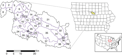
Figure 1 Study area in central Iowa and sub-watersheds in the SFIR watershed.
Download figure:
Standard image High-resolution imageFor this study, the developed model was calibrated (1996–2005 for streamflow and sediment and 2001–2005 for nitrate and phosphorus) and validated (2006–2015 for streamflow and sediment and 2006–2009 for nitrate and phosphorus). Streamflow from SWAT simulations was compared with monthly streamflow at the USGS gauging station, and monthly sediment load was estimated by using LOAD ESTimator (LOADEST) (Runkel et al 2004). The developed model consists of 39 sub-watersheds (figure 1) and 1 517 Hydrologic Response Units (HRUs). Details of input data and sources are shown in table S1 (available at stacks.iop.org/ERL/00/000000/mmedia). The land use map used four-year corn and soybean rotations, and different management operations were applied to each HRU. The auto fertilizer in SWAT was applied to the study area, whereby sufficient fertilizer was applied on the basis of the nitrogen stress for the crop growth stage (Neitsch et al 2005). This method has been used in previous studies (Baskaran et al 2010, Srinivasan et al 2010, Wu and Liu 2012, Wu et al 2013), which considered the spatial heterogeneity of soil fertilizer and provided the recommended amount of fertilizer for a specific area. In the late 1800s, subsurface tile drainage was installed in areas in the Midwest where there were poorly drained soils (Hewes and Frandson 1952). About 80% of the agricultural watershed is tile drained (Green et al 2006). In this study, tile drainage was applied to agricultural lands in the SFIR using tile drainage parameters such as depth to subsurface drain, time to drain, drain tile lag time, and depth to impervious layer in soil profile. Calibrated parameters and values are tabulated in table S2. Observed and simulated streamflow, suspended sediment (SS), NO3, and total phosphorous (TP) are shown in figure S1, and model performance for flow, SS, NO3, and TP using different statistical methods at the USGS gauging station (#05451210) are tabulated in table S3.
3.2. Riparian buffer and land conversion
Riparian buffers were developed across the major stream network in ArcGIS and simulated by using the filter strip feature in SWAT, on the basis of filter strip trapping efficiency (Neitsch et al 2005). Buffers with a filter width of 30 m were applied to adjacent water bodies. Previous studies showed the effectiveness of nitrate reduction with a 30 m buffer width (Chaubey et al 2010, Ha and Wu 2015, Mayer et al 2007, Zhang and Zhang 2011). A total of 1 508 ha of riparian area were implemented with the buffer strip, which is equivalent to 1.9% of total watershed area and 2.4% of total crop area.
As shown in figure 2(a), the intensity of land conversion to switchgrass appeared to be heterogeneous across the watershed, with a disproportional high concentration in a few sub-watersheds. The land conversion map with high energy efficiency was developed by Oak Ridge National Laboratory (Bonner et al 2014), which demonstrated the integration of switchgrass into production agriculture lands from low-productivity lands on the basis of economic analysis. A comparison of land use variations between baseline Scenario 1 and cropland conversion to switchgrass (Scenario 3) is presented in figure 2(b). In the land use conversion from idle and low-productivity areas to high-energy production lands (switchgrass), 15.2% of the entire watershed area is projected to be affected. The greatest change occurred in agricultural areas: when cropland was converted from conventional crops to switchgrass, continuous corn and corn/soybean rotation areas were reduced by 6.1% and 8.1%, respectively. Shawnee switchgrass (Trybula et al 2015) was chosen for the study area in Iowa as the appropriate species for riparian buffer areas and cropland conversion in SWAT.
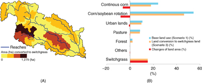
Figure 2 Land use changes in representative scenarios: (a) A map of the major stream networks and the intensity and extent of cropland conversion to switchgrass at the subbasin level (Scenarios 3, 4, 7, and 8) and (b) percent of land use in total watershed area for each land use type for Scenario 1 (baseline) and Scenario 3 (cropland conversion to switchgrass) and changes between the two scenarios.
Download figure:
Standard image High-resolution image3.3. Residue harvest and cover crop application
Biomass production and the amount of residue removal both depend on the biophysical characteristics (e.g. slope and soil properties) taken into account by specific crop management practices (Gramig et al 2013). Residue removal practices were imported by Bonner et al (2014), which described the sustainability performance of each method for residue removal, on the basis of total soil loss factor (T value reported by Soil Survey Geographic [SSURGO] Database soil map), Soil Conditioning Index (SCI) values (composite factor and organic matter factor), and annual maximum sustainable residue removal (Bonner et al 2014). For this study, supplemental nitrogen (N) and phosphorus (P) fertilizer were applied to replace nutrient loss due to residue harvest at a rate of 26.8 kg N ha yr−1 and 15.4 kg P ha yr−1 (GREET 2014). Rye was selected as the winter cover crop, with planting in October and killing in April.
3.4. Historical and future climate data
Historical precipitation and temperature data were obtained from the National Oceanic and Atmospheric Administration (NOAA) (www.ncdc.noaa.gov/cdo-web/datasets#GHCND). Climate researchers adopted Representative Concentration Pathways (RCPs) to provide a possible range of future radiative forcing values for the evaluation of atmospheric configuration (Moss et al 2008, Meinshausen et al 2011). For this study, an RCP of 4.5 (Van Vuuren et al 2011) was selected for future climate scenarios, and different projections of a moderate emission pathway were aggregated to future weather data between 2045 and 2064. The projected future climate model was obtained via downscaled CMIP5 Climate and Hydrology Projections (http://gdo-dcp.ucllnl.org/downscaled_cmip_projections). The CMIP5 is the fifth phase of the Coupled Model Intercomparison Project (CMIP) for studying the output of coupled atmosphere-ocean general circulation models (AOGCMs). The selected GCMs are ccsm4 and csiro-mk3-6-0, and a total of 12 model runs for an RCP of 4.5 were incorporated into SWAT for Scenarios 5–8; grid resolution is 1/8 degrees. To improve model performance, a bias-correction method (delta change method) was adopted for precipitation and temperature projections of the GCM, whereby the percent change in precipitation and absolute change in temperature values were calculated. Changes predicted by the GCM were averaged to monthly mean of predicted changes. These changes were perturbed into the historical observed data to generate future climate data (precipitation and temperature). Previous studies (Akhtar et al 2008, Jha and Gassman 2014, Graham et al 2007a) used the delta change methods to represent future climate precipitation and temperature data.
3.5. Water footprint
Green, blue, and grey water footprints were determined on the basis of water footprint methodology (Hoekstra et al 2011) and U.S. applications for bioenergy (Wu et al 2012a, Chiu and Wu 2012, Wu et al 2014). The water footprint measures the appropriation of fresh water amount from water consumed and/or polluted. The blue water footprint refers to the surface and groundwater consumed as part of the supply chain of a product (i.e. irrigated agriculture, industry, and domestic water use). Green water is water from rainwater not including runoff, and grey water is the amount of freshwater required to assimilate the load of pollutants to satisfy specific water quality standards (Hoekstra et al 2011). The ET value is extracted in each HRU and accumulated in each sub-watershed from the SWAT model. Calculations of grey water volume are based on background nitrate (EPA SPARROW, available at www2.epa.gov/nutrient-policy-data/nitrogen-and-phosphorus-pollution-data-access-tool) and nitrate loadings (SWAT output) at the outlet point of the SFIR watershed. On the basis of hydrology and crop growth under historical climate scenarios, a SWAT simulation showed very few water stress days and that the crops in SFIR do not need irrigation. This finding was corroborated with the 2012 Census of Agriculture for the region (USDA 2014). Therefore, blue water footprint in irrigation is zero.
4. Results and discussion
4.1. Historical and future climate data for SFIR
Historical climate data are available from 1996 to 2015 (20 years), and data for future climate scenarios are available from 2045 to 2064 (20 years). Historical and future climate data for monthly average precipitation and temperature and their changes in precipitation (%) and temperature (°C) compared with the baseline scenario (Scenario 1) are shown in figure 3. The watershed is projected to be wetter and hotter. In future climate-scenario projections, annual precipitation is 2.9% higher than the historical average, and changes in precipitation ranged from −2.3 mm (June) to 9.5 mm (May). Compared with the historical average (1996–2015), the future projected annual average temperature during 2045–2064 is 1.9 °C higher and the average growing season temperature is 1.9 °C higher. The biggest increase in monthly temperature occurs in February (2.8 °C); smaller differences were observed for the months of March, April and May (1.0 °C–1.4 °C). The projected monthly temperature for 2045–2065 in winter average 2.3 higher than 1996–2015.
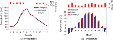
Figure 3 Monthly average precipitation (a) and temperature (b) for historical climate and projected future climate with bias correction.
Download figure:
Standard image High-resolution image4.2. Water quality
Reduction in sediment loadings (soil loss) is substantial throughout Scenarios 2–8. Land conversion to switchgrass and winter cover crop (Scenario 4) had the largest reduction in sediment loss (56.7%). Compared to the baseline scenario (Scenario 1), sediment loads were reduced by 24 030 tonnes in Scenario 2 (riparian buffer), 41 340 tonnes in Scenario 3 (cropland conversion with switchgrass), and 64 000 tonnes in Scenario 4 (stover harvest, cover crop, and cropland conversion with switchgrass) for all historical climate scenarios.
The land management strategies can result in modest reductions in nitrate loadings for the watershed. From 62 tonnes to 566 tonnes of nitrate loadings can be avoided after a riparian buffer was applied (Scenario 2), cropland was converted to switchgrass (Scenario 3), and stover was harvested and cover crop applied with cropland conversion to switchgrass (Scenario 4). The effect of land management became pronounced in Scenario 4 when land conversions to switchgrass and cover crop are implemented. As expected, phosphorus loadings follow the pattern of sediment (Demissie et al 2012, Wu et al 2012b). Phosphorous was reduced by 7.5 tonnes in Scenario 2, 3.9 tonnes in Scenario 3, and 13.8 tonnes in Scenario 4, all historical climate scenarios.
Under future climate Scenarios 5 through 8, sediment yield and phosphorus loads were reduced by up to 56.7% and 16.5%, respectively, which had the highest reduction in stover harvest, cover crop, and cropland conversion to switchgrass under future climate Scenario 8. Under Scenario 5 (base land use), sediments, phosphorus, and nitrate loading increased (figure 4). In the SFIR watershed, climate change had the greatest impact on sediment loadings (Scenario 5, no change in land use). The decrease in nitrogen loading by 34 metric tonnes in Scenario 6 (table 2; riparian buffer only), which is lower than the baseline level, is likely caused by the relatively small proportion of switchgrass in the riparian area (2.4% of crop land). With an increased scale of land conversion to switchgrass and cover crops, nitrogen loading was dramatically reduced by up to 750 metric tonnes (Scenario 8), as shown in table 2. This level of reduction has similar patterns of reduction under historical Scenario 4 (791 metric tonnes; see table 2).

Figure 4 Environmental loadings (sediments, nitrate, and total phosphorus) at SFIR watershed under land use, land management, and climate scenarios evaluated in this study.
Download figure:
Standard image High-resolution imageTable 2. (1) Stover and switchgrass harvest yield and biofuel production and (2) changes in nitrogen (N), phosphorus (P), and suspended sediment (SS) at the outlet point in the SFIR watershed for different scenarios (Scenarios 2–8), compared to the baseline scenario (Scenario 1).
| Scenarios | Harvest (metric tonnes) | Biofuel production (106L) | N change (metric tonnes) | P change (metric tonnes) | SS change (metric tonnes) | |
|---|---|---|---|---|---|---|
| Stover | Switchgrass | |||||
| 1 | — | — | — | — | — | — |
| 2 | — | 12 442 | 2.7 | −131 | −7.5 | −24 030 |
| 3 | — | 123 664 | 27.2 | −134 | −3.9 | −41 340 |
| 4 | 168 659 | 123 664 | 64.2 | −791 | −13.8 | −64 000 |
| 5 | — | — | — | 100 | 6.0 | 10 900 |
| 6 | — | 11 571 | 2.5 | −34 | −2.1 | −15 850 |
| 7 | — | 113 613 | 25.0 | −94 | 1.2 | −34 040 |
| 8 | 153 956 | 112 724 | 58.6 | −750 | −5.9 | −60 880 |
The most effective mitigation methods appeared to be those of Scenarios 3–4 and 7–8 when 15.2% of land converted to switchgrass (Scenarios 3 and 7) and land conversion are coupled with cover crops (Scenarios 4 and 8). The reduction in sediment, nitrate, and phosphorous loads in these scenarios was greater than that with the implementation of riparian buffer scenarios where 1.9% of land is converted (Scenarios 2 and 6). Results indicated that implementation of a riparian buffer and cropland conversion to switchgrass had positive effects on suspended sediment, and the level of the improvement is closely related to the area covered by switchgrass. In the watershed, wider buffer strips (i.e. up to 50 m) can be implemented to capture more nutrients and sediment.
From a biofuel production perspective, the management scenarios can yield up to 168 659 metric tonnes of corn stover and up to 123 664 metric tonnes of switchgrass for biofuel production. This amount of biomass translates to 64.2 million L (Scenario 4) and 58.6 million L (Scenario 8) of biofuel, assuming conversion yield of 80 gallons per dry ton. With cropland conversion to switchgrass (Scenario 3) at the SFIR watershed, a total of 123 664 tonnes of biomass can be produced; this amount decreased to 113 613 metric tonnes under future climate scenarios. Climate impacted crop yield differently. With future climate Scenario 8, the amount of stover that can be harvested decreased by 14 703 metric tonnes, indicating a negative impact of climate on corn yield. Also, Scenario 8 has a negative impact on switchgrass yield. Table 2 showed that the switchgrass yield decreased by about 10 940 metric tonnes (Scenario 8), compared to Scenario 4 (historical climate). The highest biofuel feedstock production was under Scenarios 4 and 8, which included switchgrass and stover harvest, compared to Scenarios 2, 3, 6, and 7. Switchgrass yields are from 7.6 to 10.2 metric tonnes/ha for scenarios 2–3 and 6–8, This shows the economical benefits that switchgrass could provide for the regional economy with moderate yield (6.72 metric tonnes/ha) and price ($50) (Brummer et al 2000).
4.3. Hydrologic components
Water availability in the watershed is represented by water yield, and water use by crops is quantified by ET. Monthly average water yield and ET with various land use scenarios and under future climate scenarios are depicted in figure 5. Land use change and cover crop shifted the water yield and ET pattern of the entire watershed. Land use change scenarios reduced water availability. Water yields under Scenario 3 and Scenario 4 are lower than the water yield under the base land use Scenario 1 throughout the year, except August through October. The hydrologic changes are closely associated with weather variables, such as precipitation and temperature. Annual precipitation and temperature increased with future climate Scenarios 5–8 compared to historical climate Scenarios 1–4. Under future climate Scenario 5, annual average water yield was increased by 18.4 mm or 6.4%. Figure 5(a) shows that more water will be available from September to May (except March), and less water will be available from June to August during crop maturation (which is closely related to decreased precipitation and increased temperature in figure S2), when water is much needed for corn in this region. Planting switchgrass on cropland (Scenario 3) increased ET by 3.3% compared with current land use, and the increase is consistent throughout the year (figure 5(b)). The largest increase in ET is predicted in September (7.4 mm for Scenario 3 and 7.7 mm for Scenario 4). Minor changes (less than 0.7 mm) are predicted during winter. With future climate Scenario 5, there is a slight increase in ET (0.5% or 3.1 mm) annually in spite of a decrease in ET in August to October. Hydrology is a non-direct process, which includes intricate interactions among ET, lateral flow, ground water, and other hydrologic components. Therefore, the water yield and ET predicted by future climate scenarios are in response to increases or decreases in precipitation and increases in temperature.

Figure 5 Monthly average water yield (a) and evapotranspiration (b) with (1) Scenario 1 (baseline land use), Scenario 3 (cropland conversion with switchgrass), and Scenario 4 (stover harvest, cover crop, and cropland conversion with switchgrass under historical climate data and (2) with the baseline land use under future climate Scenario 5.
Download figure:
Standard image High-resolution image4.4. Water footprint
Figure 6 shows the spatial distribution of green water (mm yr−1) for four different scenarios (Scenarios 1–4) at the subbasin level of the watershed. Green water is closely related to productivity of crop growth. As rain falls, it remains temporarily on top of the soil or plants. The green water footprint represents the portion of crop water demand that is satisfied by precipitation. More green water was observed upstream than downstream in the watershed. There is not a direct correlation between the green water distribution pattern (figure 6(c)) and the land conversion pattern (figure 2(a)) for Scenario 3; the distribution of green water depends more on the hydrology of the entire watershed than on the subbasin land use. However, more reductions are shown around subbasin 23 (figures 6(c) and (d)), which has the highest conversion to switchgrass figure 2(a)). At the watershed scale, Scenario 2 shows minor changes in the watershed due to small acres of riparian buffer land; there are more increases in the green water footprint in Scenarios 3 and 4.
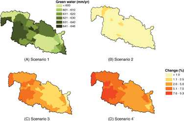
Figure 6 Green water footprint at the sub-watershed level for Scenarios 1–4 in the SFIR watershed.
Download figure:
Standard image High-resolution imageCrop residue harvesting and cover crop implementation (Scenario 4) increased green water watershed-wide. The area with the largest increase in green water is subbasin 3, which is 9.3% (48.5 mm) more than the level of green water in the baseline scenario (Scenario 1). The increase when stover is harvested (Scenario 4) could be attributable to an increase in soil evaporation or cover crop plant transpiration. As would be expected, cover crop needs water to grow. It protects soil and nutrients from running off while requiring additional ET.
The grey water footprint is derived from nitrate loadings. The nitrate grey water footprint ranged from 163 × 109 L to 222 × 109 L under historical climate scenarios and from 165 × 109 L to 234 × 109 L under future scenarios (figure 7). There is a consistent trend of decreasing grey water from riparian buffer to land conversion and then to stover harvest/cover crop planting. The degree of change is more pronounced in future climate Scenarios 5–8. Under future climate Scenario 5 (no land use change), grey water was initially increased by 5.4% compared with historical land use and then by 1.3% in Scenario 6 (the riparian buffer is implemented), and it was further increased by 2.6% in Scenario 7, when cropland is converted to switchgrass. Future Scenario 8 (switchgrass and cover crop) resulted in the greatest reduction in grey water by 25.5%. In comparison, the grey water footprint was reduced by 3.9% under Scenario 2 and 2.9% under Scenario 3, with historical climate data. Riparian buffer, cropland conversion, and cover crop scenarios evidently have positive effects on the reduction of the grey water footprint. The results of this study show that implementing land management and practices can effectively reduce the loss of sediments, nitrogen, and phosphorus in the watershed. By incorporating a riparian buffer, converting low-productivity cropland to perennials, and planting cover crop with residue harvest, the watershed has the potential of supporting cellulosic bioenergy production while improving water quality under current and future climate scenarios. Results suggest that riparian buffer and cropland conversion scenarios can be water-resource sustainable. Switchgrass is an alternative low-carbon energy source (emission reductions contribute to climate change) and needs little irrigation in most climates (i.e. good for drought conditions) (Harto et al 2010).

Figure 7 Grey water under the eight scenarios considered and a comparison with historical baseline (Scenario 1).
Download figure:
Standard image High-resolution image4.5. Stover harvest and cover crop with cropland conversion to switchgrass
Stover harvest coupled with cover crop appears to benefit water quality the most. Stover harvest rates ranged from 0.1 to 0.7 (10%–70% of the stover grown in a field were harvested) (figure 8(a)) and showed higher harvest rates upstream and relatively lower harvest rates downstream in the watershed. This result agrees with that of previous studies where simulated corn stover harvest and switchgrass planting resulted in nitrate loading reduction of up to 31% in the Upper Mississippi River basin (Wu et al 2012b) and 0%–20% in two Midwest (USA) watersheds (Cibin et al 2016). Changes of suspended sediment and phosphorous figures 8(b) and (d)) had similar patterns; there were higher reductions of each parameter (up to 2.8 t ha−1 for sediment and 0.8 kg ha−1 for phosphorous at subbasin 32) downstream of the sub-watersheds. Higher reductions in sediments and phosphorus were found at downstream subbasins 21, 22, 31, 32, 34, 35, 36, 37, and 38. These changes were quite different from the harvest rate distribution (figure 8(a)). This difference is likely caused by the implementation of a cover crop, which protects soil from runoff. Nitrate loadings are closely related to fertilizer application, and switchgrass typically requires about 50% of the fertilizer needed for corn, which means a reduction in nitrogen fertilizer input across the watershed in Scenario 3. However, stover removal also requires additional fertilizer application to supplement the nutrient loss in residue.

Figure 8 Different stover harvest rates and changes in sediment, nitrate (NO3), and phosphorous (P) under Scenario 4 (stover harvest and cover crop application with cropland conversion to switchgrass) at the subbasin level, compared to the baseline scenario (Scenario 1).
Download figure:
Standard image High-resolution image
4.6. Limitations of this Analysis
In this study, the auto fertilizer method was selected to consider spatial variation and provide proper fertilizer in the SFIR. The fertilizer rates are available at the state level (www.ers.usda.gov/data-products/fertilizer-use-and-price.aspx), which shows one fertilizer application rate representing the entire state. Specific fertilizer was applied in each HRU, which might be adequate. In reality, farmers tend to over fertilize, which is beyond the scope of this study. The delta change method is a simple bias-correction method that is straightforward to apply and uses a full range of available predictor variables. This method, however, requires normality of data, which is not useful for non-normal distribution and extreme events (Trzaska and Schnarr 2014). Sediment and nutrient transport might be sensitive to climate variability, such as extreme events.
5. Conclusion
A wide range of factors such as land use, BMPs, and climate incorporating landscape design and management concepts were examined for the SFIR watershed. Compared to baseline (Scenario 1), annual water yield (flow) was shown to decrease when cropland is converted to switchgrass (Scenarios 3 and 4) under historical climate, and increase when land use remains unchanged under future climate (Scenario 5). Green water increased when cropland is converted to switchgrass (Scenarios 2, 3, and 4) due to increased ET. Nutrient and sediment loadings decreased for the most part under riparian buffer, cover crop and land conversion to switchgrass, for both historical and future climates. Switchgrass is effective in reducing nutrients runoff. Implementing cover crop (and partial stover harvest) in combination with land use change to switchgrass (Scenarios 4 and 8) leads to the largest reduction of sediment, nitrate, and phosphorous loadings at all subbasin levels across the watershed. The two scenarios were able to produce the highest amount of biofuels from the biomass in all eight scenarios, up to 64.2 ML (Scenario 4) and 58.6 ML (Scenario 8). Results from this study enable the identification of land-use and management scenarios that could be resilient to climate change. This approach provides potentially valuable information that can aid in decision-making for planning and managing biomass development. Future study would include addressing trade-offs among water quality, production, social and economic impacts.
Notes
The authors declare no competing financial interest.
This work was supported by U.S. Department of Energy, Bioenergy Technology Office (BETO) of EERE office, under DOE ANL Contract No. DE-AC02-06CH11357. Authors thank Kara Cafferty, Ian Bonner, and Jacob Jacobson of Idaho National Laboratory for the land conversion scenario development. The authors also thank Kristen Johnson of BETO for valuable input to this study. The US government retains for itself, and others acting on its behalf, a paid-up nonexclusive, irrevocable worldwide license in said article to reproduce, prepare derivative works, distribute copies to the public, and perform publicly and display publicly, by or on behalf of the Government.