

Abstract
Given the substantial role that forests play in removing CO2 from the atmosphere, there has been a growing need to evaluate the carbon (C) implications of various forest management and land-use decisions. Although assessment of land-use change is central to national-level greenhouse gas monitoring guidelines, it is rarely incorporated into forest stand-level evaluations of C dynamics and trajectories. To better inform the assessment of forest stand C dynamics in the context of potential land-use change, we used a region-wide repeated forest inventory (n = 71 444 plots) across the eastern United States to assess forest land-use conversion and associated changes in forest C stocks. Specifically, the probability of forest area reduction between 2002–2006 and 2007–2012 on these plots was related to key driving factors such as proportion of the landscape in forest land use, distance to roads, and initial forest C. Additional factors influencing the actual reduction in forest area were then used to assess the risk of forest land-use conversion to agriculture, settlement, and water. Plots in forests along the Great Plains had the highest periodic (approximately 5 years) probability of land-use change (0.160 ± 0.075; mean ± SD) with forest conversion to agricultural uses accounting for 70.5% of the observed land-use change. Aboveground forest C stock change for plots with a reduction in forest area was −4.2 ± 17.7 Mg ha−1 (mean ± SD). The finding that poorly stocked stands and/or those with small diameter trees had the highest probability of conversion to non-forest land uses suggests that forest management strategies can maintain the US terrestrial C sink not only in terms of increased net forest growth but also retention of forest area to avoid conversion. This study highlights the importance of considering land-use change in planning and policy decisions that seek to maintain or enhance regional C sinks.
Export citation and abstract BibTeX RIS

Original content from this work may be used under the terms of the Creative Commons Attribution 3.0 licence. Any further distribution of this work must maintain attribution to the author(s) and the title of the work, journal citation and DOI.
Introduction
Forests are the world's largest terrestrial carbon (C) sink and land use is a key factor in determining the strength of this sink over time (Pan et al 2011). Globally, land management activities and land-use change (e.g. the conversion of forest land to agricultural land) released 156 Pg C to the atmosphere between 1850 and 2000 (Houghton 2003). Approximately 60% of these emissions occurred in tropical areas, primarily due to deforestation (Houghton 2003). Despite these emissions, changes in land use have been responsible for sinks in North America and Europe since the 1980s (Birdsey et al 2006, Nabuurs et al 2013). In the US, forest C accumulation has been attributed to regrowth of forests after agricultural abandonment, fire suppression, and reduced fuelwood harvesting (Albani et al 2006, Caspersen et al 2000, Houghton et al 1999). Tree growth enhancement due to CO2 fertilization, nitrogen deposition, and climate change have also contributed to the US sink (Pan et al 2009, Zhang et al 2012), but these factors in combination with others (e.g. ozone and calcium depletion) may reduce forest growth and expansion (Chappelka and Samuelson 1998, Reich 1987, Sullivan et al 2013). While environmental factors and alternative forest management strategies are important when considering C storage, this study focused on the often-overlooked risk of forest conversion to competing land uses and the associated implications on forest C stocks.
Concern about climate change has increased the monitoring of terrestrial C, which is a crucial component of national-scale reporting mechanisms under the United Nations Framework Convention on Climate Change (IPCC 2006). The Intergovernmental Panel on Climate Change (IPCC) Guidelines for National Greenhouse Gas Inventories specifically require monitoring C pools by land-use categories that include instances where land is converted from one category to another (IPCC 2006). Trends in land-use change and their correlations with environmental, political, social, and economic factors could elucidate conditions that put forests at risk of conversion to other land uses. Identifying these trends is important so that forest conservation programs (including those that have provisions for sustainable forest management) can be strategically implemented on lands of low risk of forest conversion to maximize the financial resources allocated to these programs. However, some forests in areas of high risk of conversion will be needed to maintain biodiversity and provide social benefits despite the pressure for competing land uses (e.g. the expansion of human settlement) (Pidgeon et al 2007).
The conversion of forests to specific land uses (e.g. agriculture, settlement, and lands covered or saturated by water) can be used to identify the predominant uses that result in loss of forest C stocks by country and regions within countries. A recent economic-based analysis predicted that land-use change would affect 36% of the conterminous US land area with large increases in urban land (Radeloff et al 2012). Major drivers of urban development include cultural, social, and economic factors (Fang et al 2005, Hammer et al 2004), while biophysical factors may be important drivers of change across all land uses (Martinez et al 2011). In addition to historical land-use changes, there is an increased risk of forest conversion to relatively new land uses such as cropland for ethanol production (Fargione et al 2008, Searchinger et al 2008). The creation of waterbodies through flooding also has implications for C cycling such as potentially lower rates of woody biomass decay under anaerobic conditions (Harmon et al 1986). Studies that simultaneously consider all of the potential pathways for deforested lands are needed to identify the underlying factors that make them susceptible to land-use change.
Given the dearth of empirical analysis of land-use change probability in the context of forest C dynamics, the goal of our study was to use a region-wide repeated forest inventory of the eastern US to ascertain important drivers of forest land-use conversion and forest C flux. Specific objectives included: (1) identifying the factors that were related with a full or partial reduction in forest area on re-measured plots, (2) assessing the probability of forest land conversion to agriculture, settlement, and water by region, and (3) evaluating forest C stock change on plots that experienced a reduction in forest area. Our methods are applicable to countries that have a national inventory system that includes repeated measurements of C pools and changes in land use on an existing network of permanent plots. They could also serve as a template for evaluating land-use change dynamics at multiple scales (e.g. change within specific regions). Our methods also used field-based estimates of land use and C stocks rather than remote sensing estimates, which is rare in studies of land-use change (Woodall et al 2016).
Our working hypothesis was that probability and degree of change were governed primarily by regional economic geography (i.e. the economic conditions of particular regions) given the underlying differences in primary land use patterns across the study area. For instance, forested plots within regions that have high proportions of settlement land use might have higher probabilities of forest conversion due to urban development. Also, in regions with strong cultural values tied to forest land use, the probabilities of forest conversion might be lower given the intensive use and social importance of forests. Besides the economic conditions and related social and cultural aspects of particular regions (e.g. see Alig et al 1988), we recognize that some drivers of land-use change can be common to all regions. For example, forest stands close to improved roads may have a greater risk of conversion than those further from access roads. Across all regions, poorly-stocked stands and/or those with low site productivity may have a high risk of conversion to settlement due to the motivation for short term profit rather than waiting for economic gains from future timber harvests. Conversely, forest stands with high site productivity may be converted to agricultural uses, while low productivity forests remain forested. Evaluating the correlation of these factors with land-use and C stock change involves acquiring environmental and human demographic data inclusive of the entire eastern US.
Methods
Study Area
In northern regions of the eastern US, forest types include conifer, mixed conifer, and hardwoods, whereas extensive pine (Pinus spp.) plantations and oak-hickory (Quercus-Carya) and oak-gum-cypress (Quercus-Liquidambar-Taxodium) forest types are found in southern regions (Smith et al 2009). The study area investigated here ranged westward from the state of Maine to North Dakota in the north and from Florida to Texas in the south (figure 1). This area was chosen due to the natural divide between eastern and western forests afforded by the Great Plains, which is a broad expanse of prairies, steppes, and grasslands. Across the study area, mean annual temperatures ranged from 0.5 °C to 25 °C and total annual precipitation ranged from 35 to 222 cm (Rehfeldt 2006, USFS 2016). Agriculture is the dominant land use in prairie states and along the Mississippi River valley, while forests are the dominant land use in the Great Lakes region and along most of the East and Gulf Coast regions (Woodall et al 2015b). Data collected across the study area by the USDA Forest Service Forest Inventory and Analysis (FIA) program included land condition status (e.g. forest, non-forest, and water) and non-forest land use (e.g. agricultural and settlement) on plots that were fully or partially forested (i.e. a forest condition, which was defined as having at least 10% crown cover by live trees at time of inventory or in the past based on evidence such as stumps, had to represent a portion of the plot area) (USDA 2014a). For partially forested plots, the land area in each condition was mapped by field crews during each inventory from 2002 to 2012.

Figure 1 Eastern US study area showing states (outlined in gray) and regional delineations based on US Census Bureau socioeconomic regions and National Oceanic and Atmospheric Administration climate regions (outlined in black) with the average periodic (approximately 5 years) observed probability (0–1) of forest conversion to other land uses on FIA plots within the regional delineations.
Download figure:
Standard image High-resolution imageLand use and forest inventory data
We used data (USDA 2014b) from the FIA database (USDA 2014a) that included the forest inventory of plots in 37 states of the eastern US (figure 1). The data consisted of 71 444 completely or partially forested plots (i.e. the experimental unit) established between 2002 and 2006 and re-measured approximately five years later from 2007 to 2012. Each plot consisted of four, 7.32 m fixed-radius subplots spaced 36.6 m apart in a triangular arrangement with one subplot in the center (USDA 2014a, 2014b, 2014c). All trees (live and standing dead) with a diameter at breast height of at least 12.7 cm were inventoried on forested subplots. A standing dead tree was considered downed dead wood when the lean angle of its central bole was greater than 45° from vertical. Within each sub-plot, a 2.07 m micro-plot offset 3.66 m from sub-plot center was established where only live trees with a diameter at breast height between 2.5 and 12.7 cm were inventoried. Bechtold and Patterson (2005) and USDA (2014a, 2014b, 2014c) provide more complete details regarding the FIA sample design, plot protocols, and data management.
Aboveground live and standing dead tree C stocks on the forested portions of plots were calculated using the USDA Forest Service FIA Component Ratio Method (CRM; Woodall et al 2011) to assess the influence of land-use change on measured forest C stocks (not modeled). Briefly, the CRM facilitates calculation of tree component biomass (e.g. tops and limbs) as a proportion of the total aboveground biomass based on component proportions from Jenkins et al (2003). The biomass in tree foliage was not included in our estimates of aboveground biomass. For standing dead trees, structural and decay reduction factors were applied by decay class and species (Domke et al 2011); the biomass in branches of standing dead trees was not included in this estimate. Standing dead and live total biomass was converted to C mass assuming 50% C content of woody biomass. The amount of forest area reduction that occurred on plots between inventories was calculated using the proportion of the area represented by each condition (i.e. forest, non-forest, and water) on each subplot, which were aggregated for a plot-level estimate (USDA 2014a, 2014b).
Data analysis
Binomial generalized linear modeling was used to evaluate the probability of forest area reduction on FIA plots. Data from 71 444 plots that were completely or partially forested in 2002–2006 were used to develop the binomial model. A multinomial model of land-use change from forest to agriculture, settlement, or water was also developed using data from a subset of the plots used in the binomial model (6 128 of 71 444 plots) with an actual reduction in forest area. The agricultural land-use category included croplands, pastures, idle farmlands, orchards, Christmas tree plantations, maintained wildlife openings, and rangelands. The settlement land-use category included cultural use (business and residential), rights-of-way (improved roads, railways, and powerlines), and mining use as well as undeveloped beaches and wetlands. The water land-use category included lakes, reservoirs, and ponds >0.4 ha in size, as well as streams, rivers, and canals >9 m wide. When more than one land-use change occurred on a given plot (e.g. forest to agriculture and settlement), the dominant land-use change category (according to area) was used in the multinomial model. Both models were used to quantify land-use change across all forested plots according to methods by McCullagh and Nelder (1989) and Faraway (2006) for nested responses. Specifically, rather than considering a multinomial response with four categories (forest, agriculture, settlement, and water), it was more appropriate to model land-use change as a nested response (forest remaining forest or forest conversion; with forest conversion then leading to agriculture, settlement, or water) because the majority of plots did not have a reduction in forest area (forest remaining forest). For nested responses, the likelihood of forest conversion to agriculture, settlement, and water was the product of the binomial likelihood of forest area reduction multiplied by the multinomial likelihood for the three non-forest categories conditional on forest area reduction (see the supplemental materials available at stacks.iop.org/ERL/12/024011/mmedia for an example calculation using this methodology). The glm function in the stats package and the multinom function in the nnet package (Venables and Ripley 2002) in R (R Development Core Team 2014) were used to fit the binomial and multinomial models, respectively.
For plots with a full or partial reduction in forest area, we were specifically interested in evaluating the drivers of relative forest C stock change losses and gains. Hence, separate models of C stock change were developed for plots that had negative and positive C stock change. Separate models were also developed for the total aboveground C stock (live trees ≥2.5 cm dbh and standing dead trees ≥12.7 cm dbh) and standing dead wood C stock (standing dead trees ≥12.7 cm dbh). For plots with a negative C stock change (i.e. C stock loss), the response variable was: 1−(C stock in time 2/C stock in time 1). For plots with a positive C stock change (i.e. C stock gain), the response variable was: 1−(C stock in time 1/C stock in time 2). This allowed C stock change to be compared on a relative basis with values near 1 indicating a large relative loss or gain in C stocks, respectively. A transformation, [((relative C stock change * (number of observations −1)) +0.5)/number of observations], was applied to the response variables to avoid zeros and ones (Smithson and Verkuilen 2006). Beta regression was chosen to model the response variables because the relative values for C stock losses and gains were bound between 0 and 1. The C stock change values also displayed skewed distributions that can be modeled with the beta distribution as explained by Smithson and Verkuilen (2006) and Cribari-Neto and Zeileis (2010). Models with logit and loglog links and a variable dispersion model were evaluated and the best model was selected using likelihood ratio tests and Akaike's Information Criteria (AIC) (Akaike 1972). The betareg function in the betareg package (Cribari-Neto and Zeileis 2010) in R was used to fit these models.
Numerous explanatory variables that were hypothesized as environmental, social, economic, and/or cultural drivers of land-use and C stock change were evaluated for inclusion in the statistical models (table 1). Potential landscape-level variables included: region, dominant landscape land use type (forest, agriculture, or settlement), proportion of the landscape in forest, agriculture, and settlement, distance to a landscape where settlement was the dominant land use, distance to a landscape where the proportion of the landscape in settlement was ≥0.1 (also, 0.2 and 0.3), distance to improved road, population density, and median household income. Our regional delineations were based on US Census Bureau socioeconomic regions and National Oceanic and Atmospheric Administration climate regions (figure 1). Horizontal distance from plot center to nearest improved road included paved roads and roads with gravel, grading, and ditching. Population density and income were based on US Census Bureau estimates by county in 2010. Other landscape attributes were summarized by individual 1 384 km2 hexagons as described by Woodall et al (2015b). Briefly, this hexagon size was chosen to aid in the visual interpretation of spatial patterns in C stock and land-use change. To determine the percentage of each land use type within each hexagon, the land use type at the center of each plot (median of 58 plots per hexagon) was first determined. Then, the number of plots within each land use type was summed and divided by the total number of plots in the hexagon.
Table 1. Explanatory variables used to model probability of forest area reduction (binomial model), probability of land-use change category contingent on forest area reduction (multinomial model), and relative aboveground C stock change (loss or gain), and their associated pseudo R2 values. Variables whose R2 are in bold were not highly correlated with other explanatory variables and were used in final models. Continuous variables whose R2 are in italics were not significant (P ≥ 0.05).
| Live and standing dead trees | Standing dead trees | |||||
|---|---|---|---|---|---|---|
| Variable | Binomial | Multinomial | C loss | C gain | C loss | C gain |
| Landscape-level | ||||||
| Region | 0.81 | 4.72 | 2.43 | 5.58 | 3.48 | 6.32 |
| Dominant landscape LU | 1.04 | 4.10 | 1.17 | 0.55 | 0.41 | 0.19 |
| Proportion of landscape in forest LU | 2.08 | 3.99 | 2.25 | 0.87 | 0.40 | 0.20 |
| Proportion of landscape in agriculture LU | 1.31 | 7.33 | 0.58 | 0.58 | 0.11 | 0.32 |
| Proportion of landscape in settlement LU | 1.05 | 1.38 | 2.71 | 0.36 | 0.53 | 0.03 |
| Distance to settlement as the dominant LU | 0.45 | 0.32 | 0.87 | 0.04 | 0.86 | 0.07 |
| Distance to settlement LU ≥10% | 0.74 | 0.32 | 0.87 | 0.02 | 0.23 | 0.00 |
| Distance to settlement LU ≥20% | 0.72 | 0.46 | 1.59 | 0.01 | 0.57 | 0.03 |
| Distance to settlement LU ≥30% | 0.64 | 0.34 | 1.71 | 0.04 | 1.03 | 0.30 |
| Distance to road | 3.02 | 2.22 | 0.19 | 0.01 | 0.04 | 0.07 |
| Population density | 0.22 | 1.28 | 1.43 | 0.20 | 0.31 | 0.10 |
| Median household income | 0.39 | 0.24 | 0.42 | 1.15 | 0.02 | 0.30 |
| Plot-level | ||||||
| Forest Area Reduction | — | — | 68.51 | 0.49 | 16.55 | 0.02 |
| Proportion of plot forested in T1 | 4.74 | 1.21 | 9.36 | 0.15 | 1.45 | 1.55 |
| Reserved forestland status | 0.22 | 0.37 | 0.23 | 0.10 | 0.53 | 0.03 |
| Ownership group (T1) | 1.57 | 1.70 | 1.47 | 0.45 | 0.97 | 1.20 |
| Harvest since T1 | 2.31 | 1.91 | 0.01 | 1.68 | 3.24 | 0.04 |
| Merchantable bole biomass (T1) | 1.74 | 1.45 | 9.46 | 18.66 | 0.82 | 2.10 |
| Aboveground C stock (T1) | 2.33 | 1.71 | 11.25 | 20.40 | 1.09 | 2.31 |
| Stand size class (T1) | 0.62 | 0.72 | 4.27 | 23.03 | 2.02 | 1.37 |
| Physiographic class | 0.28 | 0.39 | 0.05 | 0.02 | 0.21 | 0.08 |
| Site class productivity | 0.01 | 0.45 | 0.00 | 0.37 | 0.29 | 0.53 |
| Growth | — | — | — | 0.01 | — | 1.05 |
| Mortality | — | — | — | 6.83 | — | 0.64 |
| Water on plot (T1) | 0.00 | 1.75 | 0.43 | 0.80 | 0.02 | 0.19 |
| Slope (T1) | 0.19 | 0.00 | 1.31 | 2.06 | 0.55 | 0.35 |
T1 = time 1 (initial inventory; 2002 to 2006)
Plot-level explanatory variables considered for inclusion in the models were the proportion of the initial plot area in a forested condition, the relative amount of forest area reduction (1 − proportion of initial forest area), reserved forestland status, ownership group, the occurrence of a timber harvest between inventories, merchantable bole biomass, aboveground C stock, stand size class, physiographic class, site class productivity, tree growth and mortality, the presence or absence of a water body within plot boundaries, and slope. Reserved land was considered publicly-owned land that was permanently prohibited from being managed for the production of wood products. Land ownership categories included the US Forest Service, other federal agencies, state and local government, and private landowners. Stand size classes were based on the stocking of live trees by diameter class and included a category for plots where the stocking of live trees was <10%. Large diameter trees included hardwoods ≥27.9 cm dbh and softwoods ≥22.9 cm dbh. Medium diameter trees were considered ≥12.7 cm dbh and smaller than the large diameter trees, and small trees were considered <12.7 cm dbh. The large diameter stand size class included plots with >50% stocking in medium and large diameter trees and with the stocking of large diameter trees ≥ the stocking of medium diameter trees. If the stocking of large diameter trees was < the stocking of medium diameter trees, then the stand was classified as being in the medium diameter stand size class. Plots classified as being in the small diameter stand size class had ≥50% of the stocking in small diameter trees. Physiographic classes included hydric, mesic, and xeric conditions. Site class productivity was based on the growth potential of the stand in m3 ha−1 yr−1. Actual tree growth was calculated as the net annual growth of live trees on forest land, and mortality was calculated as the sum of the sound volume of all trees that had died between inventories. In this instance, water bodies included features such as ponds and streams <0.4 ha in size and <9 m wide that were not included in the water land-use category. For correlated explanatory variables (r ≥ | ± 0.3|), the variable with the best bivariate fit with the response variables (in terms of R2, root mean square error, and F ratio) was included in the models.
In terms of statistical limitations, we were unable to provide an estimate of error for the observed probabilities derived using the combination of binomial and multinomial models for nested responses. While some statisticians have presented modeling approaches for response categories arranged in a hierarchical format (e.g. Faraway 2006), the methods used to calculate error terms for observed probabilities are usually not presented. To our knowledge, McCullagh and Nelder (1989) are the only statisticians that have examined, in detail, error associated with such probabilities. They present two approaches for modeling pneumoconiosis in coalminers; one approach uses ordinal regression (to model categories of disease severity) and an alternative approach involving two nested responses derived from binomial models (risk of having the disease and risk of having severe symptoms). The authors present standard errors for both approaches, but they do not provide detailed numerical calculations for the alternative approach. Furthermore, in most examples of nested responses the explanatory variables are the same for all models. Hence, we are unaware of how this would influence the calculation of error terms. While we believe that our study provides a straightforward approach to quantifying the probability of forest conversion, future studies that quantify the uncertainty associated with our modeling approach would be valuable.
Results
Observed trends
Nine percent of the completely or partially forested FIA plots evaluated in this study (6 128 of 71 444) had a reduction in forest area between 2002–2006 and 2007–2012. Ninety-nine percent of plots with a reduction in forest area occurred in the managed forest landscape (i.e. non-reserve status). For plots in managed forest landscape, aboveground forest C stock change for plots with a reduction in forest area was −4.2 ± 17.7 Mg ha−1 (mean ± SD) compared with 2.3± 15.2 Mg ha−1 for plots with no reduction or gains in forest area (table 2). Across all non-reserved plots (i.e. not designated as federal wilderness) with a reduction in forest area, total aboveground forest C stock change was −1 723 Mg compared with 8 980 Mg for non-reserve plots with no reduction or gains in forest area (table 2). Average relative forest area reduction was greatest on plots where the dominant land-use change was from forest to agriculture (0.436) compared with land-use change from forest to settlement or water (0.299 and 0.244, respectively). For reserve plots, forest conversion to water accounted for 69% of the observed land-use change.
Table 2. Average and standard deviation (in parentheses) aboveground (live tree and standing dead wood) and standing dead wood C stock change (Mg ha−1) for plots with a reduction in forest area and without a reduction or gain in forest area between 2002–2006 and 2007–2012. Also shown are changes in total C stock (Mg) across all plots within each reserve status and land-use change category (i.e. the summation of C stock change values for plots within each category).
| Forest area reduction | No forest area reduction or gain | |||
|---|---|---|---|---|
| Non-reserve (N = 6 042) | Reserve (N = 86) | Non-reserve (N = 57 376) | Reserve (N = 2 149) | |
| Aboveground C stock change (Mg ha−1) | −4.2 (17.7) | −1.8 (15.3) | 2.3 (15.2) | 2.0 (9.6) |
| Total aboveground C stock change (Mg) | −1 722.9 | −10.4 | 8 980.3 | 286.6 |
| Standing dead wood C stock change (Mg ha−1) | −0.2 (2.5) | 0.2 (1.7) | 0.1 (2.7) | 0.4 (4.2) |
| Total standing dead wood C stock change (Mg) | −74.7 | 1.0 | 305.9 | 61.0 |
N = number of plots
Land-use change
The proportion of the landscape in forest land use, distance to road, aboveground C stocks, and the interaction between distance to road and aboveground C stocks explained 6.7% of the deviance in the probability of forest area reduction (table 3). The probability of reduction in forest area was highest where non-forest land uses dominated the landscape, distance from plot center to road was minimal, and aboveground C stocks were high (figure 2). Deviance in the probability of forest area reduction was also explained by the proportion of the plot area in a forested condition in 2002–2006 (i.e. at the time of the first inventory) (figure S1), with the highest probability of forest area reduction occurring on plots with minimal area in a forested condition. However, it was not included in the binomial model because it was correlated with the proportion of the landscape in forest land use (r = 0.26), distance to road (r = 0.15), and aboveground C stocks (r = 0.34).
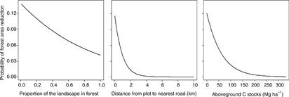
Figure 2 Periodic (approximately 5 years) observed probability (0–1) of forest area reduction on FIA plots while holding other explanatory variables in the binomial model constant at their mean values (proportion of the landscape in forest land use = 0.70, distance to road = 0.623 km, aboveground C stocks = 42.5 Mg ha−1).
Download figure:
Standard image High-resolution imageThe proportion of the landscape in agricultural land use, population density, distance to road, aboveground C stocks, the presence or absence of a water body within plot boundaries, and several interaction terms explained 13.4% of the deviance in the probability of land-use change to agriculture, settlement, or water conditional on forest area reduction (table 3). The presence or absence of a water body within the plot boundaries mainly resulted in shifts between the observed probabilities of land-use change to agriculture versus water (figure 3). A regional variable was not included in the multinomial model because it was correlated with the proportion of the landscape in agricultural land use, but it alone explained 4.7% of the deviance in land-use change. In the model with region (representing regional economic and climatic conditions) as the only explanatory variable, the New England and Southeast regions had the highest probability of land-use change to settlement (table S1).
Table 3. Parameter estimates (standard errors in parentheses) for quantifying the probability of forest area reduction (binomial model) and land-use change category (agriculture, settlement, or water) contingent on forest area reduction (multinomial model).
| Parameter | |||||||
|---|---|---|---|---|---|---|---|
| Model | b0 |
b1 | b2 | b3 | b4 | b5 | b6 |
| Binomial | −0.7423 (0.0425) | −1.3195 (0.0534) | −0.5190 (0.0531) | −0.0087 (0.0007) | −0.0144 (0.0016) | — — | — — |
| Multinomial (settlement) | 1.2264/1.2356 (0.0716/0.0792) | −3.2968 (0.1394) | 0.0006 (0.0001) | −0.2008 (0.0920) | 0.0138 (0.0015) | −0.0011 (0.0002) | −0.0060 (0.0026) |
| Multinomial (water) | −2.5088/−1.0696 (0.1489/0.1205) | −0.5051 (0.2334) | 0.0001 (0.0001) | 0.3574 (0.0978) | 0.0128 (0.0024) | −0.0001 (0.0003) | 0.0034 (0.0026) |
ln (probability of forest area reduction) = b0 + b1(forest) + b2(road) + b3(C stocks) + b4(road) (C stocks); forest, proportion of the landscape in forest (0–1); road, distance from plot to nearest road (km); C stocks, aboveground C stocks (Mg ha−1). ln (probability of land-use category = settlement (or water), given agriculture as the baseline) = b0 + b1(agriculture) + b2(population) + b3(road) + b4(C stocks) + b5(population)(road) + b6(road) (C stocks); agriculture = proportion of the landscape in agriculture, population = population density (people km−2). aFor the multinomial equations, the first parameter estimate listed for the intercept (b0) was used when small water bodies were not present within plot boundaries and the second estimate was used when small water bodies were present.

Figure 3 Panels showing the influence of each continuous variable and the absence or presence of a water body within plot boundaries on the periodic (approximately 5 years) probability (0–1) of land-use change type (agriculture, settlement, water) conditional on forest area reduction, while holding other explanatory variables in the multinomial model constant at their mean values (proportion of the landscape in agriculture = 0.28, population density = 440 people km2, distance to road = 0.314 km, aboveground C stocks = 31.2 Mg ha−1).
Download figure:
Standard image High-resolution imageThe binomial and multinomial models were jointly used to quantify the probability of forest land conversion to agriculture, settlement, and water. The average observed probability of forest land conversion to agriculture was the highest for the Plains and Iowa/Missouri regions (0.108 and 0.057, respectively) (table 4). The average observed probability of forest land conversion to settlement was highest in southern New England and the Southeast (0.066 and 0.058, respectively), and lowest in northern New England and the Plains (0.042 and 0.039, respectively). The average observed probability of forest land conversion to water was highest for the Plains and Iowa and Missouri regions (0.013 and 0.010, respectively). The Plains region had the highest overall risk of forest land conversion to other land uses (0.160) (figure 1, table 4).
Table 4. Average and standard deviation (in parentheses) of observed probabilities (0–1) of forest land conversion to agriculture, settlement, and water on FIA plots by geographic region based on the combined results of binomial and multinomial models.
| Region | N | Agriculture | Settlement | Water | Overall |
|---|---|---|---|---|---|
| Northern New England | 4 671 | 0.011 (0.009) | 0.042 (0.026) | 0.003 (0.003) | 0.057 (0.035) |
| Southern New England | 919 | 0.010 (0.010) | 0.066 (0.042) | 0.003 (0.003) | 0.078 (0.047) |
| Mid-Atlantic | 6 415 | 0.018 (0.019) | 0.053 (0.037) | 0.004 (0.005) | 0.076 (0.052) |
| Southeast | 15 685 | 0.022 (0.020) | 0.058 (0.031) | 0.004 (0.004) | 0.084 (0.045) |
| South | 13 587 | 0.025 (0.023) | 0.053 (0.028) | 0.004 (0.005) | 0.082 (0.046) |
| Ohio Valley | 10 069 | 0.035 (0.038) | 0.053 (0.031) | 0.007 (0.008) | 0.095 (0.059) |
| Iowa and Missouri | 3 628 | 0.057 (0.050) | 0.048 (0.025) | 0.010 (0.010) | 0.116 (0.064) |
| Upper Mid-West | 15 280 | 0.031 (0.034) | 0.049 (0.029) | 0.005 (0.006) | 0.086 (0.056) |
| Plains | 1 190 | 0.108 (0.065) | 0.039 (0.023) | 0.013 (0.011) | 0.160 (0.075) |
N = number of plots
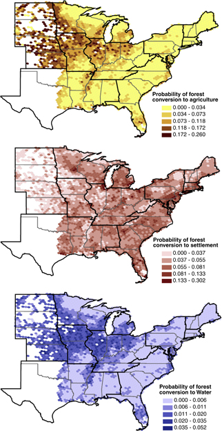
To facilitate interpretation of spatial patterns in land-use change across the study area, we averaged the observed probabilities of forest conversion to other land uses for the plots of this study that were within the 1 384 km2 hexagons developed by Woodall et al (2015a). The average observed probabilities of forest conversion within hexagons visually reinforces regional trends in the data (figure 4). However, as stated above, other variables besides regional economic geography explained more deviance in the probability of forest conversion to other land uses, which makes our models applicable across the entire study area while simultaneously capturing regional differences in land-use change.
Figure 4 Average periodic (approximately 5 years) observed probability (0–1) of forest conversion to agriculture, settlement, and water on FIA plots within individual 1 384 km2 hexagons. White hexagons (primarily in the Plains states) did not include FIA plots that were forested at the time of the initial inventory (2002–2006); also, western portions of Oklahoma and Texas were not included in the analysis.
Download figure:
Standard image High-resolution image
Forest carbon dynamics
For plots that experienced a reduction in both forest area and aboveground C stocks, relative aboveground (live trees + standing dead wood) C stock loss was best explained by the relative amount of forest area reduction (pseudo R2 = 68.5%). Not surprisingly, greater reduction in forest area on plots tended to be associated with higher losses in aboveground forest C stocks. Deviance in aboveground C stock loss was also explained by aboveground C stock and ownership group in 2002–2006 (pseudo R2 = 11.3 and 1.5%, respectively). Plots with high aboveground C stocks, which were typically associated with US Forest Service lands, tended to have the lowest relative C loss. However, aboveground C stock in 2002–2006 was correlated with forest area reduction (r = −0.35), so aboveground C stock and ownership group were not included in the model of aboveground C stock loss.
For plots that experienced a reduction in forest area and an increase in aboveground C stocks, relative aboveground C gain was best explained by stand size class (pseudo R2 = 23.0%). Deviance in forest C stock gain was also explained by aboveground C stock in 2002–2006 and tree mortality between inventories (pseudo R2 = 20.4 and 6.8%, respectively), but were not included in the model because of their correlation with stand size class. Plots with less than 10% stocking of live trees and dominated by trees in the smaller diameter classes, which typically had low aboveground C stocks and limited tree mortality, tended to have higher relative C gains. The average observed relative aboveground C gains for the large diameter, medium diameter, small diameter, and poorly-stocked plots were 0.146 ± 0.115, 0.213 ± 0.152, 0.456 ± 0.306, and 0.539 ± 0.356 (mean ± SD), respectively. There were also clear differences in C stock gain by regional economies, which alone explained 5.6% of the deviance in relative aboveground C stock gain. The highest observed gains tended to be in the South and Southeast (table 5).
Table 5. Average and standard deviation (in parentheses) of observed relative aboveground C stock gain (1−(C stock in time 1/C stock in time 2)) and loss (1−(C stock in time 2/C stock in time 1)) on FIA plots that experienced both a reduction in forest area and an increase or decrease in aboveground C stocks, respectively, by region and C stock (live and standing dead trees combined, and standing dead trees); absolute values (Mg ha−1) are also shown.
| Region | N (C stock loss) | Relative C stock loss | Absolute C stock loss | N (C stock gain) | Relative C stock gain | Absolute C stock gain |
|---|---|---|---|---|---|---|
| Live and standing dead trees | ||||||
| Northern New England | 83 | 0.418 (0.349) | −17.6 (17.2) | 102 | 0.210 (0.194) | 5.0 (4.1) |
| Southern New England | 50 | 0.555 (0.370) | −20.8 (19.1) | 44 | 0.128 (0.103) | 5.0 (3.5) |
| Mid-Atlantic | 236 | 0.568 (0.392) | −18.9 (20.6) | 239 | 0.187 (0.191) | 5.1 (4.1) |
| Southeast | 656 | 0.612 (0.385) | −20.4 (23.2) | 734 | 0.321 (0.277) | 8.5 (7.4) |
| South | 533 | 0.629 (0.371) | −17.4 (18.8) | 573 | 0.347 (0.286) | 8.1 (7.0) |
| Ohio Valley | 507 | 0.528 (0.400) | −15.0 (18.7) | 517 | 0.204 (0.186) | 5.8 (4.6) |
| Iowa and Missouri | 186 | 0.506 (0.384) | −12.6 (14.8) | 195 | 0.169 (0.159) | 3.7 (3.1) |
| Upper Mid-West | 421 | 0.458 (0.373) | −11.1 (15.8) | 619 | 0.210 (0.196) | 4.1 (3.5) |
| Plains | 87 | 0.610 (0.378) | −10.9 (15.3) | 85 | 0.168 (0.116) | 3.1 (2.7) |
| Standing dead trees | ||||||
| Northern New England | 93 | 0.742 (0.319) | −1.5 (2.6) | 56 | 0.627 (0.366) | 0.8 (1.5) |
| Southern New England | 47 | 0.793 (0.279) | −1.2 (2.0) | 21 | 0.667 (0.335) | 1.2 (1.8) |
| Mid-Atlantic | 172 | 0.761 (0.281) | −1.3 (2.3) | 124 | 0.744 (0.333) | 1.3 (1.9) |
| Southeast | 473 | 0.822 (0.276) | −1.8 (2.9) | 263 | 0.805 (0.298) | 1.4 (2.1) |
| South | 342 | 0.863 (0.244) | −2.1 (3.5) | 190 | 0.865 (0.245) | 1.4 (2.2) |
| Ohio Valley | 352 | 0.757 (0.307) | −1.6 (3.0) | 265 | 0.745 (0.315) | 1.7 (3.4) |
| Iowa and Missouri | 130 | 0.732 (0.312) | −1.9 (2.8) | 101 | 0.729 (0.332) | 2.3 (3.7) |
| Upper Mid-West | 373 | 0.696 (0.341) | −1.3 (2.3) | 367 | 0.678 (0.316) | 1.8 (3.0) |
| Plains | 49 | 0.763 (0.317) | −1.9 (3.3) | 45 | 0.822 (0.272) | 2.4 (2.5) |
N = number of plots
For plots that experienced both a reduction in forest area and a decrease in aboveground standing dead wood C stocks, relative aboveground standing dead wood C loss was best explained by the relative amount of forest area reduction (pseudo R2 = 16.6%). Similar to the findings for the combined live and dead C stocks, greater reduction in forest area was associated with high standing dead wood C loss. Deviance in relative standing dead wood C stock loss was also explained by the proportion of the plot in a forested condition and aboveground C stock in 2002–2006 (pseudo R2 = 1.5 and 1.1%, respectively). Relative C stock losses tended to be associated with plots with a low proportion of forest area and low aboveground C stocks. Also, plots in the South had the highest observed relative and absolute standing dead wood C stock loss compared to other regions (table 5).
For plots that experienced a reduction in forest area and an increase in aboveground standing dead wood C stocks, relative aboveground standing dead wood C gain was best explained by regional economies (pseudo R2 = 6.3%). The South and Southeast regions had the highest relative gains, while the Iowa/Missouri, Upper Mid-West, and Ohio Valley regions had the highest absolute gains; the Plains states had both high relative and absolute gains compared to other regions (table 5). Deviance in relative standing dead wood C stock gain was also explained by stand size class and ownership group (pseudo R2 = 1.4 and 1.2%, respectively). The largest C stock gains tended to occur on plots with low stocking or those dominated by small diameter trees, and on private and federal lands besides National Forests.
Discussion
While identifying forest management strategies that maximize C storage in forests is important, forest management decisions should also be considered in the context of land-use change. Our study provides a methodology for evaluating the probability of forest land conversion to competing land uses, which could be used in conjunction with simulations of forest C stocks under different management strategies. In our analysis that involved plots with a reduction in both forest area and aboveground C stocks, greater C stock loss occurred on plots with a greater amount of forest area reduction, which highlights the importance of maintaining forest area. On plots with a reduction in forest area and aboveground C stock gains, stand size class and regional economies were associated with aboveground C stock gains. The highest observed gains tended to be in the South and Southeast, likely due, in part, to climatic factors (e.g. long growing seasons and warm temperatures) associated with high live tree biomass production and C sequestration (Brown and Schroeder 1999). Overall, these results suggest keeping forest as forest is important, regardless of which forest management strategies are employed.
Considering our working hypothesis that land-use change was primarily driven by regional economic geography, we found that these were generally associated with forest conversion to other land uses, in part, through their correlation with the proportion of landscape in forest and agricultural land uses. Correlated factors captured regional trends such as the high observed probability of forest conversion to agricultural uses in the Plains states. We speculate that forest conversion to cropland for corn used in ethanol production could have been a primary driver of this change as indicated by other studies (Fargione et al 2008, Searchinger et al 2008). Northern New England, which was dominated by the forest land use, had the lowest observed probability of forest conversion. This could be related to ownership by entities whose primary objective was timber management and to the enrollment of forested lands in state programs that aim to preserve working forests. In addition, plots in landscapes with a high proportion of non-forest land use had the highest probability of forest conversion, which suggests that forests in fragmented landscapes have a high risk of conversion.
Distance from plot to nearest road, the presence of a small water body (i.e. a water body <0.4 ha in size or a stream <9 m wide) within the forested portion of the plot, and aboveground C stocks were also correlated with forest conversion to other land uses. For plots with a reduction in forest area and <1 km from the nearest road, the primary land-use change was from forest to settlement, which is likely related to the expansion of human settlements (Hammer et al 2004, Pidgeon et al 2007, Radeloff et al 2005). As the proportion of the landscape in agriculture increased, so did the probability of land-use change to water. The presence of small water bodies also increased the likelihood of land-use change to water. This may be related to expansion of small (<0.1 ha) agricultural impoundments that were once used for irrigation or livestock watering, or the creation of larger (≥0.4 ha) impoundments for these uses (Powers et al 2013). In remote areas (i.e. as distance from plot to the nearest road increased), forest conversion was primarily to large water bodies. After their extirpation from many regions of North America, beavers (Castor canadensis) are now increasing and their influence on stream and river hydrology may partially explain forest conversion to large water bodies including ponds and lakes and the widening of streams and rivers in remote areas (DeGraaf and Yamasaki 2003, Naiman et al 1994).
The low probability of forest area reduction on plots with high aboveground C stocks is due, in part, to observations in protected areas (e.g. wilderness areas) and perhaps forests enrolled in C offset or conservation programs that have high live and dead tree biomass pools. Landowners may be more willing to convert forests with low aboveground C stocks to other land uses because profits from timber harvesting may not be realized in the short term (Poudyal et al 2014). Interestingly, forest conversion on plots with high aboveground C stocks was primarily due to settlement with the average amount of forest area reduction accompanying land-use change due to settlement being less than when land-use change was due to agricultural conversion. This may be related to landowners' attraction to and desire to retain forest land with large trees and other natural amenities on a portion of their properties (Hammer et al 2004).
Plots that were poorly stocked and those dominated by small-diameter trees had the highest aboveground forest C stock gains, despite partial forest area reduction. However, plots with these stand attributes also had the highest risk of forest conversion to other land uses. This suggests that forest management strategies that maintain adequate stocking of medium- to large-diameter trees may be at less risk to conversion to non-forest land uses. On plots with both a reduction in forest area and standing dead wood C stocks, the highest observed standing dead wood C stock losses were in the South. This was likely due to windthrow or bole breakage of snags during Hurricane Katrina in 2005, which occurred during the inventory re-measurement period. On plots with a reduction in forest area and standing dead wood C stock gains in the mid-western US regions, observed standing dead wood C stock gains may be the result of tree mortality due to the emerald ash borer (Agrilus planipennis). In addition, stands without reductions in forest area and hence less exposure to winds may be less susceptible to windthrow of live and dead trees (Foster and Boose 1992).
Despite the extensive geographic and temporal extent of the data and the reliance on field-based estimates rather than remote sensing, the analysis does have some important limitations as previously discussed elsewhere (Coulston et al 2014, Woodall et al 2016). First, the temporal period examined has strong economic variability that may greatly influence the observed trends. Financial indicators were evaluated and did not show strong relationship to the observed trends. Second, better information about C pools on non-forest lands, such as C stored in soils and urban trees, is needed to evaluate C dynamics when land-use transitions occur (Woodall et al 2015a). Third, increased land-use resolution (especially non-forest) may elucidate drivers of land-use change. For example, the identification of cropland used for ethanol production within the agricultural category could confirm our hypothesis of forest conversion to cropland in the Great Plains and adjacent regions. Within regions, models that quantify the probability of afforestation could be coupled with models of forest land-use change risk to provide land managers with tools for forecasting forest C storage potential across land uses. Our results indicate that the specific type of land-use change could also be used to estimate the amount of forest reduction or afforestation that would accompany changes in land use. Fourth, as noted in the description of our study's methods, analyses such as those developed in our study would benefit from rigorous uncertainty assessments. Finally, our models could be used to improve the accuracy of models that predict land-use change using probability surfaces (e.g. the FORE-SCE model). For instance, our observed probabilities of land-use change could be used as baseline information for FORE-SCE model projections such as those made by Sohl et al (2014) and Zhao et al (2013).
Conclusion
Our study one was of the first to simultaneously consider dynamics of land-use change and forest attributes in the determination of C dynamics at the stand-level. For regions in the eastern US, it was found that the Great Plains had the highest probability of forest conversion. The overriding determinant of aboveground forest C stock loss was the amount of forest area reduction that occurred on plots with its condition being subordinate. Major drivers of forest land-use change risk were the proportion of the surrounding landscape in a forested condition, distance to nearest road, and aboveground forest C stocks. Human population density and the presence of water bodies were also correlated with the specific type of land-use change that occurred. While geographic region based on differences in regional economies and climatic conditions was not included in our models of land-use change, other factors that were correlated with these conditions were capable of robustly capturing regional trends and differences, suggesting broader application of the developed models. In terms of advantages of forest management strategies for maintaining the US terrestrial C sink, forest stands that were poorly stocked and/or with small diameter trees had the highest probability of conversion to non-forest land uses. As a comprehensive view of forest C (land-use context and forest management) may be needed to ensure maintenance of the forest C sink in the eastern US, the detailed monitoring of land use coupled with advances in terrestrial C monitoring (e.g. soil organic C across land uses) is paramount. Finally, forest management tools that include land-use change risks should be developed to enable forest management decision making when the ecosystem service of C storage is one of the primary concerns.
Acknowledgments
We thank Daniel Hayes (University of Maine), Liu Shuguany (US Geological Survey), and three anonymous reviewers who provided useful comments that helped us to improve this manuscript. We also thank Paul Sowers (US Forest Service) for consolidating data from the FIA database that were used in this analysis. We also acknowledge Brian Walters (US Forest Service) for providing spatial data and their associated attributes. Funding for this project was provided by the US Forest Service as part of a Joint Venture Agreement between the University of Maine and the US Forest Service (#14-JV-11242305-053). This is Scientific Contribution no. 3507 of the Maine Agricultural and Forest Experimentation Station.