

Abstract
We performed an intercomparison of river discharge regulated by dams under four meteorological forcings among five global hydrological models for a historical period by simulation. This is the first global multimodel intercomparison study on dam-regulated river flow. Although the simulations were conducted globally, the Missouri–Mississippi and Green–Colorado Rivers were chosen as case-study sites in this study. The hydrological models incorporate generic schemes of dam operation, not specific to a certain dam. We examined river discharge on a longitudinal section of river channels to investigate the effects of dams on simulated discharge, especially at the seasonal time scale. We found that the magnitude of dam regulation differed considerably among the hydrological models. The difference was attributable not only to dam operation schemes but also to the magnitude of simulated river discharge flowing into dams. That is, although a similar algorithm of dam operation schemes was incorporated in different hydrological models, the magnitude of dam regulation substantially differed among the models. Intermodel discrepancies tended to decrease toward the lower reaches of these river basins, which means model dependence is less significant toward lower reaches. These case-study results imply that, intermodel comparisons of river discharge should be made at different locations along the river's course to critically examine the performance of hydrological models because the performance can vary with the locations.
Export citation and abstract BibTeX RIS

Original content from this work may be used under the terms of the Creative Commons Attribution 3.0 licence.
Any further distribution of this work must maintain attribution to the author(s) and the title of the work, journal citation and DOI.
Corrections were made to this article on 25 April 2017. The supplementary data was updated.
1. Introduction
Humans have constructed approximately 60 000 dams and reservoirs worldwide (Avakyan and Iakovleva 1998, ICOLD 2016) with the aim of providing stable access to water resources and preventing riverine disasters. Humans also use riverine water for irrigation, and municipal and industrial purposes. Currently, most of the world's large rivers are regulated by dams (Nilsson et al 2005). To simulate river discharge affected by human impacts worldwide, global hydrological models (GHMs) implementing dam regulation and water abstraction schemes are necessary (Biemans et al 2011, Bierkens 2015, Nazemi and Wheater 2015a, 2015b).
Hydrological simulations are subject to uncertainties arising from various factors. Among them, uncertainties from meteorological forcings and hydrological models are predominant. Firstly, the various global meteorological data sets compiled from observed data with various compilation methodologies may contain different atmospheric conditions (including precipitation), which affects simulated runoff and river discharge (e.g. Müller Schmied et al 2016a).
Secondly, hydrological models themselves are also sources of uncertainty. Each model implements different schemes for land surface processes (e.g. runoff, evapotranspiration, and infiltration) or river routing processes and also uses different parameters. As a result, even simulations of natural flow (unregulated flow without water withdrawal) differ considerably among GHMs (Haddeland et al 2011). Moreover, human interventions in river flow, such as dam operation and water withdrawal from surface water bodies (e.g. rivers and lakes) and groundwater, are additional sources of uncertainty among GHMs. Although a variety of dam operation strategies exist to meet local water resource requirements/uses, weather conditions, social/political demands and so forth, operational rules and historical records of operations are not available to the public except for a limited number of cases. Therefore, present GHMs incorporate generic schemes of dam operation (e.g. Hanasaki et al 2006, Haddeland et al 2006). Hereafter, the term 'generic schemes' indicates schemes that are not specific to a certain dam but are applicable to a group of dams. Such schemes fundamentally shift the timing of outflows by temporarily storing water without changing the total volume of river flow, insofar as evaporation from open water surfaces of dam reservoirs is considered to be secondary. Generic schemes can successfully reduce errors of simulated river discharge compared with observed discharge. However, practical application of these schemes to actual riverine management has room for further improvement due to their simplification of dam functions (Hanasaki et al 2006).
With the rising use of GHMs, it has become increasingly important to examine their performance through intercomparison (Haddeland et al 2011, Schewe et al 2014, Gosling et al 2016), as well as in terms of water withdrawal (Wada et al 2013) and extreme hydrological events (Dankers et al 2014, Prudhomme et al 2014). However, no intercomparison of flow regulation has been performed. Moreover, since river flow can be regulated by multiple dams in a river channel, the differences in flow regulation among GHMs should be systematically investigated. In this study, the impacts of dam operation on river flow are examined from upstream to downstream. In addition, it is important to compare simulated and observed discharges to check the model performance in hydrological simulations. For global-scale simulations, comparisons have often been performed at one or a few representative gauge stations for each basin (Nijssen et al 2001, Sperna Weiland et al 2010, Hattermann et al 2017). The station which has a long history of observation near the furthest main-stem reach is favorably used because river flow at these locations is considered to reflect the overall characteristics of the basin. However, since highly regulated rivers have variable seasonal behavior, even among river sectors separated by dams, comparisons and validations of river flow at the furthest reach is insufficient to identify sources of intermodel differences. It is important to perform intercomparisons of regulated river flow by decomposing river channels into sectors from the upper to lower reaches, similar to the longitudinal section analysis of Vörösmarty et al (1997).
In this paper, we simulated of river discharge under multiple meteorological forcings for the historical period of 1971–2000 using multiple models and examined the characteristics of river discharge regulated by dams. The objectives of this paper are twofold. (1) We examine the effects of different models by comparing the simulated seasonality of river discharge obtained using five GHMs (section 3.1). Here, we compare the alteration of river flow by dams at the seasonal timescale obtained with multiple models. (2) We also discuss discrepancies among the models under multiple forcings (section 3.2). To elucidate the effects of dam regulation, we examine the Missouri-Mississippi and Green–Colorado river simulations as case studies. This research was performed under the framework of Phase 2a of the Inter-Sectoral Impact Model Intercomparison Project (ISIMIP).
The structure of this paper is as follows. We outline the data sets and analytical methods in section 2. The results are presented in section 3. We discuss the performance and potential problems of the regulated river flow simulations in section 4. In section 5, the conclusions are presented.
2. Data and Methods
2.1. Historical meteorological data
Four historical meteorological data sets were used in this study, namely GSWP3 (Kim et al 2014), Princeton PGMFD ver2 (Sheffield et al 2006), WFDEI.gpcc (Weedon et al 2014) and WATCH (Weedon et al 2010), hereafter referred to as GSWP3, PGFv2, WFDEI and WATCH, respectively (table 1). Since WFDEI.gpcc covers 1979 onward, WFDEI is a combination of WATCH (before 1979) and WFDEI.gpcc (after 1979) in ISIMIP2a. Meteorological variables used in this simulation depend on GHMs (see table A1 stacks.iop.org/ERL/12/055002/mmedia), employing different land process schemes. Müller Schmied et al (2016a) examined these meteorological data sets and pointed out that differences in chronological decadal trends of meteorological variables caused differences in simulated discharge and evapotranspiration.
Table 1. Historical meteorological data sets used in this study. The last column shows whether wind-induced precipitation undercatch is corrected. These data sets were re-gridded and distributed by the ISIMIP.
| Data sets (Abbreviation) | Reanalysis | Precipitation correction | Undercatch |
|---|---|---|---|
| GSWP3 | 20th Century |
GPCC ver6, CRU TS3.21 | Corrected |
| Princeton PGMFD ver.2 (PGFv2) | NCEP-NCAR |
CRU TS3.21 | Uncorrected |
| WFDEI.gpcc (WFDEI) | ERA-Interim |
GPCC ver5/6 | Corrected |
| WATCH | ERA-40 |
GPCC ver4 | Corrected |
aCompo et al (2011) bKalnay et al (1996) cDee et al (2011) dUppala et al (2005)
2.2. Hydrological simulations
We used the following five GHMs: DBH (Tang et al 2007), H08 (Hanasaki et al 2008a, 2008b), LPJmL (Rost et al 2008, Biemans et al 2011), PCR-GLOBWB (Wada et al 2014) and WaterGAP (Müller Schmied et al 2014, 2016a). All GHMs included dam operation (in consideration of construction year) in their simulation. Their results were available on January, 2016, in the ISIMIP2a framework. In the main, the model settings followed ISIMIP2a protocol (ISIMIP, 2015), although there were some exceptions. All the models covered the globe at a resolution of 0.5° × 0.5° for the period 1971–2000, which is common simulation periods determined by the ISIMIP protocol for the four meteorological data sets. The hydrological state variables of each model at the beginning of 1971 were stabilized (spun-up) using pre-1970 data. River routing was achieved using DDM30 (Döll and Lehner 2002) (see section 2.4 later). Analysis settings and model specifications are briefly summarized in table 2 and online supplementary table A1.
Table 2. Hydrological models used in this study. Abbreviations for water use: (Ir) irrigation, (D) domestic, (In) industry, (Mn) manufacturing, (Lv) livestock, and (C) cooling of thermal power plants. See also table A1 for other specifications of each model.
| GHM | Water use | Calibration | River routing | Dam operation scheme | Evaporation from water surface of dams |
|---|---|---|---|---|---|
| DBH | Ir | No | linear reservoir, DDM30 | Hanasaki et al (2006) |
No |
| H08 | Ir,D,In | No | linear reservoir, DDM30 | Hanasaki et al (2006) |
No |
| LPJmL | Ir,D,In,Lv | No | linear reservoir, DDM30 | Biemans et al (2011) | Considered |
| PCR-GLOBWB | Ir,D,In,Lv | No | travel-time routing | Wada et al (2014) | Considered |
| WaterGAP | Ir,D,Mn,Lv,C |
Calibrated on long-term mean annual discharge |
linear reservoir, DDM30 | Hanasaki et al (2006) |
Considered |
aFor WaterGAP, Mn + C = In. bCalibration covers 54% of global land surface, according to Müller Schmied et al (2016a). cSee also supplement A2.
To examine anthropogenic effects on river flow, we used simulations called 'varsoc' runs, defined by ISIMIP2a, which included time-varying human interventions (standard analysis settings were dams, water withdrawal, and changes in land use over basins; see also tables 2 and A1 for details). Historical land use (e.g. type of crop cultivation) is represented annually by Dynamic MIRCA-HYDE. This is a historical extension of MIRCA2000 (Portmann et al 2010), which provides land use data circa 2000 with the extension of time-varying trends given by HYDE3.1 (Goldewijk et al 2011). Dam specifications (location, storage capacity, and construction year) were provided by GRanD ver. 1.1 (Lehner et al 2011a, 2011b). Essentially, the GHMs implemented the dam location data provided as standard data by ISIMIP, which was georeferenced to DDM30. We also used 'nosoc' runs in naturalized, control simulations, in which neither human withdrawals nor dam operation were considered.
Some GHMs used analysis settings that were different from the standard ones. As shown in table 2, four of the five models included human withdrawals other than irrigation. WaterGAP adopts static land use but varies irrigation areas yearly. Regarding the dam location data, some GHMs relocated dams in consideration of different priorities (table A2; see also comparison maps by Müller Schmied et al (2016b)).
2.3. Post-simulation analysis
In this paper, we focused mainly on the climatological seasonality of river discharge for two major global rivers, and compared simulated data with observations. We aggregated both simulated and observed daily river discharge over three-month periods: December to February (DJF), March to May (MAM), June to August (JJA), and September to November (SON), which correspond to winter, spring, summer, and fall, respectively.
The observed discharge data were obtained from the archive of the Global Runoff Data Centre (GRDC) and the United States Geological Survey (USGS). To compare simulated and observed discharge, we georeferenced the river gauge station to DDM30 so that the catchment area of the station agreed with that of DDM30. We divided the analysis period 1971–2000 into three 10-yr time spans in our analysis because not all gauge stations had been in operation over the entire 30-yr analysis period. To utilize as many gauge stations as possible for comparison with simulated discharge and to suppress meteorological year-to-year variability, we considered the 10-year period is adequate for our purpose.
2.4. Case studies
In this paper, the Missouri-Mississippi and Colorado River basins were chosen as case studies. We chose these river basins because (1) historical river discharge records are available, particularly for gauge stations in different river sectors separated by large dams, (2) there is clear seasonality in the river discharge, (3) the flow is significantly regulated by large reservoirs, and (4) both river basins have large catchment areas so that differences in geographical characteristics inside these river basins can be resolved at a resolution of 0.5° × 0.5°. In fact, the levels of flow regulation are 15.5% and 280% for the Mississippi and Colorado River Basins, respectively, estimated as the percentage of total reservoir capacity within a river system relative to volumetric annual discharge, following Nilsson et al (2005) (table S1). Moreover, historical reservoir operation records for major dams on these rivers are available. In this study, we performed both multiforcing and multimodel comparisons for the Missouri-Mississippi River and a multimodel comparison for the regulated flow of the Green–Colorado River.
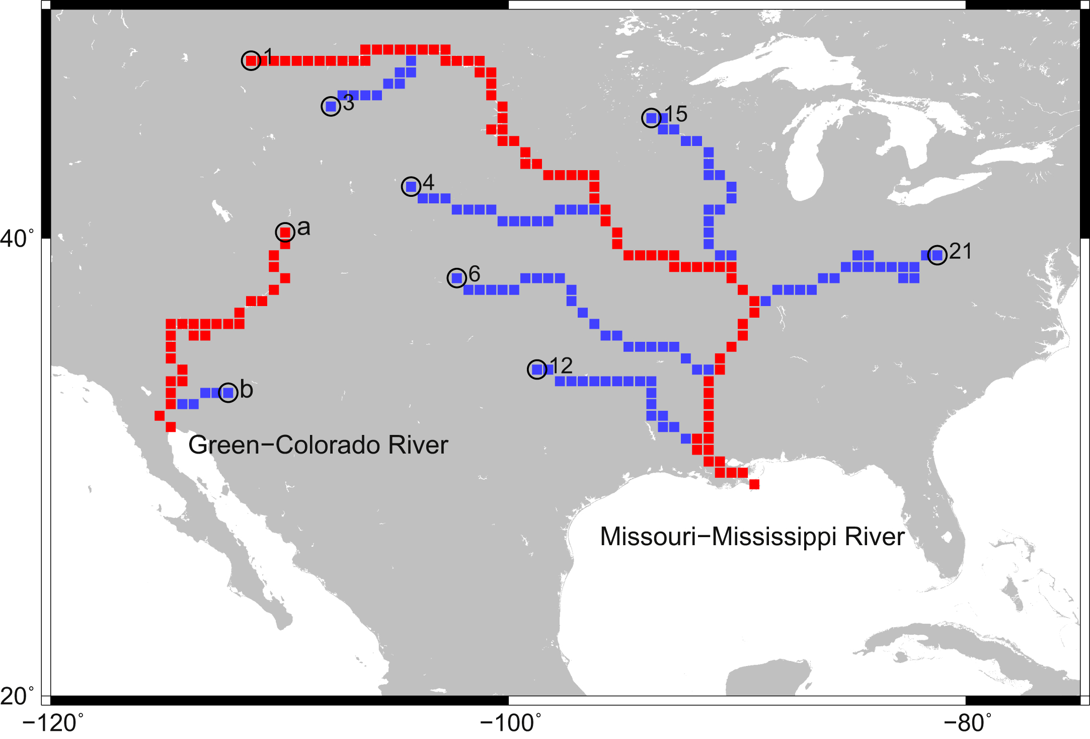
To analyze discharge on a longitudinal section of these rivers, we allocated the sequential cell number (SCN) along the main channel from the upper to the lower reaches (figure 1) of these rivers. Figure 1 also shows the land cells with simulated annual mean river discharge (varsoc run) >100 m3 s−1 for each GHM. Since these major rivers have high water flux, land cells with low discharge (those in dark gray in figure 1) were not considered as part of the main stem in each GHM.

Figure 1 Example of major river channels implemented in each global hydrological model (GHM) in the central part of the United States. Black grid lines separate land cells with the dimensions of 0.5° × 0.5°. To visualize the channels, symbols were added to the land cells with an annual average discharge (varsoc run) of greater than 100 m3 s−1. Different symbols were marked for each GHM (see the inserted box). The numbers superimposed on the land cells show the sequence of land cells along the longest stems of the Missouri–Mississippi (flowing from the top center to the bottom right in the map) and Green–Colorado (from the center to bottom left) Rivers. Owing to the instability of hydrological simulation over a small catchment area, we omitted the first 10 cells of the river from the source in the intermodel comparison.
Download figure:
Standard image High-resolution image2.4.1. Missouri–Mississippi River Basin
The Mississippi River is (including its tributaries) the third largest river basin in the world and travels through a wide range of climates and geography from snow-packed mountainous areas to temperate plains. The flow has clear natural seasonality due to spring snowmelt in the mountainous areas and heavy rain in the plains during warm months, but is heavily regulated by large dams on the Missouri River.
Large dams have been constructed since the mid-20th century to maintain the riverine environment. Five large dams (table A3) have significant impacts on seasonal river flow due to their large storage capacity (see US Army Corps (2006) for dam management details). In this study, historical dam operation data obtained from the US Army Corps of Engineers (Northwest Division) were also used in the analysis. To compare simulated and observed discharges, 12 gauge stations (table A4 and fig. A1) along the Missouri–Mississippi River were used.
2.4.2. Green–Colorado River Basin
The Colorado River starts in the Rocky Mountains, travels through a dry region, and flows into the Gulf of California. The river is known to be one of the most regulated rivers in the world (Glen Canyon and Hoover Dams; see table A5). We chose this basin expecting that uncertainty in operation schemes would be clearly detected in simulated river discharge because of the high ratio of the dam capacity to the annual discharge. Moreover, the water is also supplied for irrigation and municipal use in the basin and its neighborhood. Thus, hydrological simulation using a generic dam operation scheme in this river basin is not only challenging, but also useful to examine intermodel discrepancies due to dam operation. Historically, the discharge of this river system was drastically changed by the construction of the Hoover Dam (storage: 3.670 × 10¹⁰ m3) in 1935 and Glen Canyon Dam (storage: 2.507 × 10¹⁰ m3) in 1963. The peak river flow in the upper basin occurs in spring due to snowmelt. Note that the Green River is also regulated by Flaming Gorge Dam (storage: 4.336 × 10⁹ m3).
We focused on a longitudinal section along the Green and Colorado Rivers, the longest reach of the river system. Five gauge stations (table A6) were used for comparison.
3. Results
3.1. Intercomparison of the seasonal fraction of river discharge among hydrological models
The seasonal fraction of river discharge varied among the GHMs. To visualize the effects of dam operation on the seasonal flow at different river sectors fragmented by dams, we drew a longitudinal section along each river channel (sections 3.1.1 and 3.1.2) and interpreted the results with hydrographs (section 3.1.3). In this section, we used the simulation results forced by GSWP3 for simplicity. Since the seasonality of main channel flow is altered not only by dams but also by the confluence of major tributaries under natural conditions, we also accounted for major tributaries in the interpretation (see also figure 2).

Figure 2 Major tributaries (indicated in blue) directly flowing into the Missouri–Mississippi or Green–Colorado Rivers (red). IDs were assigned to each tributary. The individual river names are: (1) Missouri, (3) Yellowstone, (4) Platte, (6) Arkansas, (12) Red, (15) (Upper) Mississippi, and (21) Ohio for the Missouri–Mississippi River System, and (a) Green and (b) Gila for the Green–Colorado River System. Only river sectors more than 10 cells from the source are indicated.
Download figure:
Standard image High-resolution image3.1.1. Missouri–Mississippi River
Figure 3 shows the results of the seasonal fraction of discharge for the Missouri–Mississippi River. The horizontal axis gives the location along the main stem in terms of the SCN from the upper (leftward) to lower (rightward) reaches. For each GHM, seasonal fractions relative to annual discharge are shown, with corresponding heights presented in different colors. Although only river discharge for the decade 1971–1980 is shown, similar seasonality was observed in other decades. Figure 4 extracts the seasonal fractions at three representative sites on the channel from figure 3 for intermodel comparison.
Among the GHMs, a high flow was generally observed in spring-summer due to mountain snowmelt in the upper reaches. As the river flows down to the plains, the climate becomes warmer and precipitation increases, peaking in summer. An evenly distributed flow throughout the seasons can be observed in the middle reach of the Mississippi River. Seasonal behavior also changes downstream from the confluence of tributaries, such as the Arkansas (#6), (Upper) Mississippi (#15) and Ohio (#21) Rivers. In the lower reaches of the Mississippi River, water is abstracted for irrigation (figure C2 includes only the results from H08), but withdrawal is sufficiently smaller than the river discharge so it did not markedly alter the river flow seasonality.
The intermodel comparison of river flow seasonality frequently showed the greatest proportion of river flow in spring to summer, but the seasonal fraction of river flow differed among the GHMs (figures 3 and 4). H08 had higher flow in spring, whereas DBH had higher flow in summer. Note that high annual variations can be seen in the upper reaches, whereas there were lower annual variations among the GHMs in the lower reaches.
Next, we focused on flow regulation by dams. Judging by the discontinuity in the seasonal fraction of river flow due to the impact of dams (e.g. Fort Peck Dam at SCN 22), the magnitude of seasonal flow regulation differed markedly among the GHMs. H08, LPJmL, and WaterGAP introduced greater seasonal flow modulation than DBH and PCR-GLOBWB. Intermodel differences in seasonality were weakened as the river flowed downstream, possibly because of flows merging according to various seasonal behaviors of tributaries. The seasonality of the five-GHM ensemble mean reproduced the seasonality observed at land cells where gauge stations were located. However, discontinuity at dams was unclear as a result of averaging. Moreover, whether regulated flows began in land cells where dams were located, or in an adjacent cell, depended on the GHM.
Based on the observed seasonality at the gauges, each model has advantages and disadvantages with respect to reproducing seasonality along the whole channel (table C1). Even if a GHM performs well for some river sectors, it does not perfectly reproduce seasonality for other river sectors. Note that the seasonality of WaterGAP was not explicitly affected from calibration because WaterGAP was calibrated with long-term mean annual discharge, not seasonal discharge.

Figure 3 Seasonal fraction of river discharge simulated using five hydrological models (varsoc run) and basic hydroclimatological parameters (runoff and evapotranspiration by H08) on a longitudinal section along the Missouri–Mississippi River. The horizontal axis gives the sequential cell number (SCN) from the uppermost reach of the Missouri River (as indicated in figure 1). (a) Historical changes in precipitation, evapotranspiration, and runoff are shown as blue, green, and red lines for 1951–1960, 1971–1980, and 1991–2000, respectively. Tributaries that meet the Missouri–Mississippi River are indicated by numbers in the upper panel. See also Tributary IDs in figure 2. (b) The seasonal fraction of river flow for 1971–1980 is indicated by different colors: cyan (DJF), green (MAM), orange (JJA), and magenta (SON). Gray cells indicate land cells through which the river channels used by each GHM did not pass (see figure 1). The observed seasonality at gauge stations is indicated by the ladder-shaped boxes. White broken lines show equal partitions among seasons (25% each). (c) Dam capacity is indicated in the same colors as (a). Fort Peck (F), Garrison (G), and Oahe (O) Dams are located at SCNs 22, 33, and 42, respectively.
Download figure:
Standard image High-resolution image
Figure 4 Intermodel comparison of seasonal fraction of river discharge, shown in figure 3, at three selected sites on the Missouri–Mississippi River. Three sites are representative of the upper (SCN 12), middle (SCN 50) and lower (SCN 90) reaches. The seasonal fractions of river flow for 1971–1980 are indicated by different colors: cyan (DJF), green (MAM), orange (JJA), and magenta (SON). The outermost circle represents the ensemble mean of the five GHMs.
Download figure:
Standard image High-resolution image3.1.2. Green–Colorado River
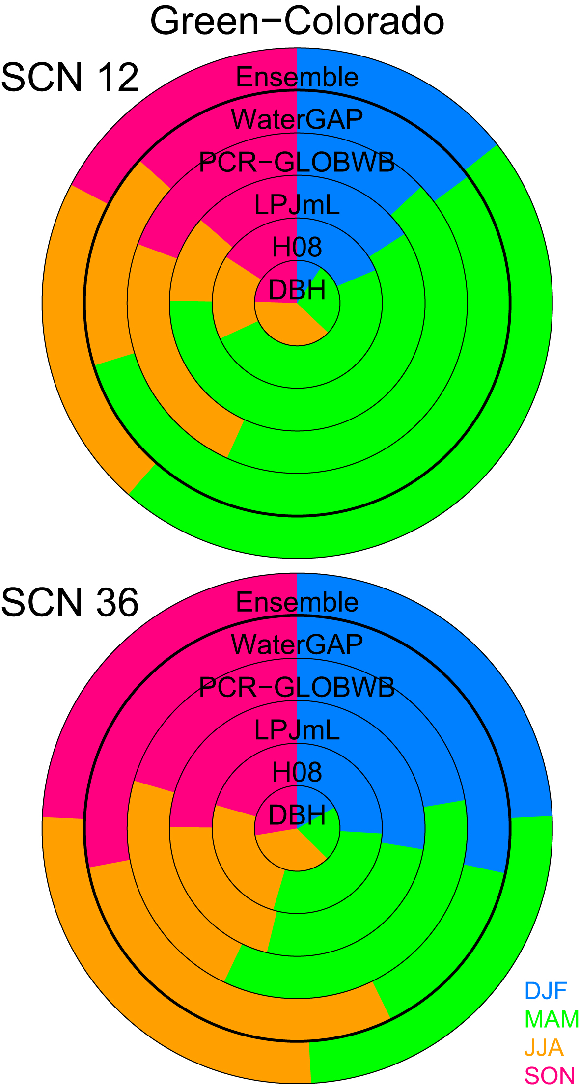
Figure 5 shows the results for the Green–Colorado River for 1971–1980. Since the seasonality of the observed river discharge changed somewhat over the decades, we also included the results for 1991–2000 in the Supplement (figure C1). The seasonal fractions at two representative sites on the channel are shown in figure 6. As mentioned earlier, reproducing the seasonal flow of the Colorado River is challenging for all hydrological models, owing to multiple human interventions. The simulated discharge of the Green River tended to be higher in spring than in other seasons, whereas the observed discharge was higher in both spring and summer. At Glen Canyon Dam (SCN 17) in the Colorado River, the seasonal flow variation was markedly reduced. All the GHMs showed less seasonality toward the river mouth. In the lower reaches, river water was abstracted for irrigation (which can also be seen in figure C3 in the results for H08), but the withdrawal was sufficiently small compared with the river discharge. Thus, irrigation was hardly noticeable in the river flow seasonality.
The magnitude of flow regulation at the dams differed among the models. H08, LPJmL, and WaterGAP showed strong flow regulation, whereas the other models showed weaker regulation. The five-GHM ensemble mean reproduced the observed seasonality with reasonable accuracy. We note that discontinuity in the seasonality simulated with WaterGAP at the three cells from the lowermost reach was generated by strong calibration of the simulated discharge (reduced to ca. 25%), intended to match the long-term mean of the observed annual discharge. This feature was also observed as a sudden decrease in annual discharge at SCNs 36–38 in figure 1.

Figure 5 Same as figure 3 but for the longitudinal section along the Green–Colorado River, with river discharge data for 1971–1980. The horizontal axis gives the SCN from the uppermost reach of the Green River (as indicated in figure 1). Glen Canyon (C) and Hoover (H) Dams are located at SCNs 17 and 28, respectively.
Download figure:
Standard image High-resolution image
Figure 6 Intermodel comparison of the seasonal fraction of river discharge shown in figure 5 at two selected sites on the Green–Colorado River. Two sites are representative of the upper (SCN 12) and lower (SCN 36) reaches. A similar representation to figure 4 is used.
Download figure:
Standard image High-resolution image3.1.3. Different magnitudes of flow regulation across GHMs
These results showed that flow regulation differed considerably across the GHMs. What explains these differences? We examined their causes by using simulated hydrographs at sites downstream of large dams (Fort Peck Dam in the Missouri River and Glen Canyon Dam in the Colorado River). We focused on how the river flow was modulated by the dams in each GHM. For this purpose, we analyzed land cells where the dams are located in each GHM because the location could differ by one cell upstream or downstream along the main channel among the GHMs.
Tables 3 and 4 show mean river discharge at the dam sites. The ranges of the forcing-ensemble means among the GHMs were markedly larger than those of the GHM-ensemble means among the meteorological forcings. The ranges of the final columns were 725.3 m3 s−1 for Fort Peck Dam and 669.9 m3 s−1 for Glen Canyon Dam, whereas those of the final rows were 105.6 m3 s−1 and 227.3 m3 s−1, respectively. These results indicate that the spread of the simulated river discharge depended more strongly on the GHM than on the meteorological forcing, which is consistent with published intercomparison studies using multiple general circulation models and multiple GHMs (e.g. Wada et al 2014, Hattermann et al 2017). These large intermodel differences in mean discharge were not attributable to the variations in catchment area that resulted from differences in the dam locations used by the GHMs. If we re-evaluate the range of mean river discharge at the common land cell (SCN 22 for Fort Peck Dam and SCN 17 for Glen Canyon Dam, following the standard dam data distributed by ISIMIP, the intermodel ranges (725.3 m3 s−1 for Fort Peck Dam and 642.2 m3 s−1 for Glen Canyon Dam) are still larger than the interforcing ranges (112.1 m3 s−1 and 229.0 m3 s−1, respectively).
Figure 7 shows hydrographs and cumulative discharge at the dam sites (note that a plot of the cumulative discharge of natural flow with a longer time is known as a mass curve or Rippl diagram, which is useful for designing the dam capacity (Rippl 1883, Adeloye 2012)). By comparing regulated flow with natural flow, we found that seasonal variability was suppressed by dam regulation, i.e. decreased discharge in the high-flow season and increased discharge in the low-flow season. As a result, the mass curve in the high-flow season (spring to summer) had a more gradual slope and less curvature for regulated flow than for natural flow.
DBH gave larger estimates of the mean river discharge for 1971–1980 than the other GHMs (figure 7; tables 3 and 4). Since the effective magnitude of flow regulation by dams is given approximately by the ratio of dam capacity to mean annual discharge, DBH regulates river flow more weakly than the other models. This is one reason why the flow regulation was marginal in DBH. On the other hand, the mean discharge of LPJmL at Glen Canyon Dam was comparable to that of DBH (table 4). However, the hydrographs (figure 7) showed that its seasonal peak flow was larger and lasted for a shorter duration than LPJmL. The clear seasonal contrast in the LPJmL simulation helped the dam to act as a stronger regulator than it did in the DBH simulation.
The magnitude of flow regulation at the seasonal scale was not determined principally by the dam manipulation scheme adopted by each GHM. Although DBH, H08, and WaterGAP implemented the flow regulation scheme proposed by Hanasaki et al (2006), the simulated flow regulation contrasted clearly between DBH (with weak regulation) and H08 or WaterGAP (with strong regulation). Dam outflow is primarily determined as a function of the mean annual inflow in the scheme of Hanasaki et al (2006) (see A1 in the Supplement). Therefore, simulated variables such as dam water storage at the beginning of the operational year, water demand (dams for irrigation purposes only), inflow variability, and the consequent differences in water storage are considered as the actual causes of the discrepancies in seasonal-scale dam flow regulation among the GHMs.
Table 3. Mean river discharge at Fort Peck Dam for 1971–1980. The numbers in brackets show the turnover (detention) period required to fill the nominal dam capacity (2.356 × 10¹⁰ m3) at the rate of the mean river discharge.
| GHM | SCN | GSWP3 | PGFv2 | WFDEI | WATCH | Ensemble | |||||
|---|---|---|---|---|---|---|---|---|---|---|---|
| m3 s−1 | (d) | m3 s−1 | (d) | m3 s−1 | (d) | m3 s−1 | (d) | m3 s−1 | (d) | ||
| DBH | 22 | 832.4 | (327.6) | 914.2 | (298.3) | 1137.7 | (239.7) | 1157.1 | (235.7) | 1010.4 | (269.9) |
| H08 | 22 | 275.6 | (989.4) | 218.9 | (1245.7) | 322.3 | (846.1) | 323.9 | (841.9) | 285.1 | (956.5) |
| LPJmL | 21 | 454.3 | (600.2) | 495.7 | (550.1) | 614.0 | (444.1) | 618.3 | (441.0) | 545.6 | (499.8) |
| PCR-GLOBWB | 22 | 415.2 | (656.8) | 402.5 | (677.5) | 401.0 | (680.0) | 383.4 | (711.2) | 400.5 | (680.9) |
| WaterGAP | 21 | 287.5 | (948.5) | 327.1 | (833.6) | 295.4 | (923.1) | 310.4 | (878.5) | 305.1 | (893.8) |
| Ensemble | 453.0 | (602.0) | 471.7 | (578.1) | 554.1 | (492.1) | 558.6 | (488.2) | 509.3 | (535.4) | |
Table 4. Mean river discharge at Glen Canyon Dam for 1971–1980. The numbers in brackets show the turnover (detention) period required to fill the nominal dam capacity (2.507 × 10¹⁰ m3) at the rate of the mean river discharge.
| GHM | SCN | GSWP3 | PGFv2 | WFDEI | WATCH | Ensemble | |||||
|---|---|---|---|---|---|---|---|---|---|---|---|
| m3 s−1 | (d) | m3 s−1 | (d) | m3 s−1 | (d) | m3 s−1 | (d) | m3 s−1 | (d) | ||
| DBH | 17 | 849.7 | (341.5) | 1024.2 | (283.3) | 1349.4 | (215.0) | 1386.5 | (209.3) | 1152.5 | (251.8) |
| H08 | 17 | 549.4 | (528.1) | 600.2 | (483.4) | 772.0 | (375.9) | 797.8 | (363.7) | 679.8 | (426.8) |
| LPJmL | 19 | 882.1 | (328.9) | 1056.8 | (274.6) | 1151.2 | (252.1) | 1150.8 | (252.1) | 1060.2 | (273.7) |
| PCR-GLOBWB | 17 | 590.9 | (491.1) | 700.3 | (414.3) | 667.2 | (434.9) | 632.9 | (458.5) | 647.8 | (447.9) |
| WaterGAP | 18 | 447.1 | (649.0) | 487.9 | (594.7) | 507.8 | (571.4) | 487.6 | (595.1) | 482.6 | (601.2) |
| Ensemble | 663.8 | (437.1) | 773.9 | (374.9) | 889.5 | (326.2) | 891.1 | (325.6) | 804.6 | (360.6) | |

Figure 7 Hydrograph and cumulative discharge (so-called mass curve or Rippl diagram) based on the mean daily discharge for 1971–1980 at a site downstream of Fort Peck and Glen Canyon Dams. Green and black lines show the results of the nosoc (without human influences) and varsoc (with water withdrawal and dam regulation) runs. The horizontal axis is the day of the year (DOY in calendar year). The meteorological forcing is GSWP3. Horizontally aligned panels show the results of each GHM. From left to right, DBH, H08, LPJmL, PCR-GLOBWB, and WaterGAP. The location (shown as SCN) is indicated in each panel.
Download figure:
Standard image High-resolution image3.2. Differences in the seasonal fraction of river discharge under four meteorological forcings
The discrepancies in flow regulation among the GHMs also varied with the rivers' courses. To quantify the variance in the seasonal fraction of river discharge among the five GHMs, we calculated the standard deviation (SD) of the five GHMs from their ensemble mean for each season under four meteorological forcings. Figures 8 and 9 show the results for the Missouri–Mississippi and Green–Colorado Rivers, respectively. Since the seasonal fraction is a normalized value by the annual discharge, the fraction is comparable with ones at different locations.
Three major characteristics were observed in the results for the multiple GHMs and forcings. First, the obtained SDs were generally independent of the meteorological forcing for a large proportion of the river sectors. This indicates that SDs were explained primarily by differences among GHMs rather than meteorological forcings. This finding is consistent with tables 3 and 4 at the two selected sites. Second, larger SDs were observed more frequently in upper reaches than in lower reaches: SDs generally decreased downstream. This means that even if GHMs generally agree in the lower reaches, larger discrepancies may still exist in the upper reaches. Third, SDs in absolute terms tended to be larger during high-flow seasons (spring to summer for both rivers) than during low-flow seasons (fall to winter).

Figure 8 Standard deviations (SDs) of the seasonal fraction of river discharge in the longitudinal section along the Missouri–Mississippi River among the five GHMs. The seasonal fraction for each GHM is shown in figure 3. The horizontal axis is the SCN from the uppermost reach of the Missouri River (as indicated in figure 1). Meteorological forcing data sets are indicated by different colors: purple (GSWP3), red (PGFv2), blue (WFDEI), and green (WATCH). Results of the varsoc and nosoc runs are shown by filled circles and crosses, respectively. Blank cells indicate that SDs were not calculated because of missing data for some GHMs. Fort Peck (F), Garrison (G), and Oahe (O) Dams are located at SCNs 22, 33, and 42, respectively.
Download figure:
Standard image High-resolution image
Figure 9 Same as figure 8 but for the longitudinal section along the Green–Colorado River. The seasonal fraction for each GHM was shown in figure 5. The horizontal axis is the sequential cell number (SCN) from the uppermost reach of the Green River (as indicated in figure 1). Glen Canyon (C) and Hoover (H) Dams are located at SCNs 17 and 28, respectively.
Download figure:
Standard image High-resolution image
Next, we examined the differences in the results between natural and regulated flows. Overall, natural flow (crosses) tended to have slightly higher SD values than regulated flow (filled circles) for MAM, JJA, and SON. This implies that implementing dam regulation schemes contributes to small discrepancies among the GHM results. Large intermodel discrepancies in natural flow were observed more frequently in high-flow seasons than in low-flow seasons (e.g. figure 7) because of high variability in precipitation events. Dams contributed to a flattening of the variability and redistribution of water among the seasons, which lowered the SD of regulated flow during high-flow seasons. By contrast, the regulated flow for DJF had slightly higher SD values than the natural flow in some river sectors. Winter had the lowest discharge for both rivers because of the accumulation of snowpack in mountainous areas and the weak rainfall over the catchment area. Thus, a stable and low flow was observed for all the GHMs, along with a similar temporal profile. Dam operation in low-flow seasons increased the discharge, but its amplification was different among the GHMs (figure 7). This explains the larger SDs for regulated flow compared to natural flow for DJF.
Note that these findings did not always hold true. For example, at Fort Peck Dam (SCN 22) on the Missouri–Mississippi River (figure 8), the SD of the regulated flow discontinuously increased downstream for DJF but decreased for MAM and SON. Because flow seasonality drastically changed into less seasonal variability by the dam (figure 3), MAM seasonal fraction of discharge converged among the GHMs, even though MAM was a high-flow season for natural flow.
4. Discussion
4.1. Interpretation of hydrological simulation of river discharge regulated by dams
In this study, we examined the uncertainties among GHMs and the potential errors along river channels and obtained new insights and caveats through case studies for the interpretation of simulated river discharge specific to regulated rivers.
First, differences in the seasonal fraction were detected among the GHMs. This is likely attributable to two factors: natural flow and dam regulation. (1) Regarding natural flow, differences among the GHMs were expected based on previous studies (e.g. Haddeland et al 2011). Moreover, difficulties in reproducing snowmelt may also be a source of intermodel differences because both river basins used in this study are covered by a thick snowpack in winter (e.g. Slater et al 2001, Rutter et al 2009). In fact, over the catchment areas of Fort Peck Dam and Glen Canyon Dam, winter precipitation occurs as snow (figures B1 and B2, respectively). Small differences in meteorological conditions (especially temperature) triggering snow melt can result in divergence in the timing of floods.
(2) Regarding dam regulation, dams fundamentally alter the timing of flow without changing absolute volumes of water when the dam capacity is large compared to the mean annual flow, and when secondary effects (local inflow to the dam, evaporation loss from the water surface, withdrawal or diversion for water supply and so forth) are regarded as sufficiently small compared with river flow. That is, the long-term average annual volume of discharge is considered to be independent of the dam operation scheme. To the best of our knowledge, generic dam operation schemes are fundamentally based on a function of inflow to the dam and the water demand for each purpose of the dam (Hanasaki et al 2006, Haddeland et al 2006). Recall that the natural inflow was different among the GHMs. Even if the same dam capacity was adopted for multiple GHMs, differences in dam inflows can cause simulated river discharge to diverge downstream among the GHMs due to different responses to the simulated inflow.
There are intrinsic difficulties in constructing advanced generic schemes for dam regulation. Dam operation data are generally not publicly available. The dams along the Missouri River represent a very rare case in which the operation strategy is publicly available (US Army Corps 2006). Although the actual operation of multiple dams in the same river basin is more complex because they are mutually linked (e.g. Nagy et al 2002), this is not taken into account by the operation schemes implemented in the GHMs.
In this study, we used the seasonal fractions of river flow, not the absolute seasonal volumes, because Haddeland et al (2011) revealed that annual river discharge values also differ among GHMs with a wide range of runoff coefficients (runoff divided by precipitation) at the basin scale. By introducing the seasonal fraction normalized by the annual volume, we expect that seasonal dam operation behavior can be focused on by artificially cancelling the effect of differences among runoff coefficients.
Secondly, the case studies also showed decreasing intermodel differences moving toward the lower reaches. This probably reflects the fact that averaging over a larger catchment area helps stabilize simulated river discharges, which are susceptible to local instabilities. In most hydrological analyses, the performance of a simulation is evaluated at gauge stations at the farthest reach of the river, because river flow there reflects the overall characteristics of the catchment area, namely, the whole river basin. This is convenient for obtaining an overall picture of the basin. However, we should keep in mind that larger intermodel discrepancies may exist at gauge stations upstream.
In this paper, we only discussed two case-study river basins. However, notice that we used only simulated river discharge, one of fundamental variables in hydrological simulations, to depict dam functions. Visualizing methods like figures 3 and 5 are applicable to other river basins in the world, if river discharge data are available.
GHMs will play an increasingly important role in evaluating hydrological impacts on societies as global climates and environments change rapidly, because they can simulate water availability with human interventions at the global scale under given meteorological conditions. Currently, most rivers flowing through populated areas are regulated by dams. In the future, GHMs will still strongly rely on generic dam operation schemes to make them applicable at the global scale.
Both river discharge and storage in dams have been attracting interest. For example, hydropower generation is increasingly seen as a means of reducing the emission of greenhouse gases while meeting the increasing demand for electricity. Hydrological simulation can also be used to assess the future potential of hydropower generation (e.g. Lehner et al 2005, Masaki et al 2014, Liu et al 2016). Moreover, large dams create an anaerobic environment at the bottom and emit methane to the atmosphere, especially in tropical regions (Fearnside 1995, Abril et al 2005, Kemenes et al 2007). From an ecological viewpoint, aquatic environments and ecosystems are of great concern. Physical aspects (e.g. surface area, level, and storage) of the water surface are observed with various techniques, such as remote sensing imagery, satellite altimetry, and bathymetry, to study aquatic environments. Accurate estimation of dam storage using GHMs will be welcomed not only by hydrological scientists, but also by those in the related fields of environmental and social sciences.
4.2. Future improvement of GHMs with regulated rivers
There is a considerable trade-off, specific to GHMs, in pursuing global applicability and high-performance reproductions of observed river discharge at the cost of ignoring local diversity in the natural and social environments of each river basin. In practice, GHMs with a spatial resolution of 0.5° × 0.5° can neither consider all local conditions nor implement dam operation schemes for the over 60 000 dams across the world. This is in clear contrast to regional hydrological models (RHMs), which can be tuned to a certain river basin and its environment, and can potentially implement an actual dam manipulation scheme. We consider there to be no essential differences between GHMs and RHMs in terms of model structure, analytical scheme, and the physics of hydrological processes, as summarized in table A3 of Hattermann et al (2017). Moreover, as discussed in detail in Hattermann et al (2017), the high performance of RHMs is considered to be partly due to calibration, which poses the simultaneous risk of over-calibration. In addition, Gosling et al (2016) found little difference in the simulations from an ensemble of GHMs and an ensemble of RHMs, when the individual models were forced with meteorological projections from climate models.
Despite such a trade-off relationship, high-accuracy reproduction of the world's river discharge using GHMs should be the ultimate goal to improve our understanding of surface waters. Multimodel intercomparison studies carried out in the last several years have revealed broader differences among GHMs. It is critical to examine the reasons for this, identify sources of error, and improve models (e.g. Huber et al 2014), as is being attempted currently. As we showed in this study, dam regulation is a source of differences among GHMs. Amending these models would result in high-performance simulations and greatly benefit hydrological science.
Some of our intercomparison results are degraded because of inconsistencies in simulation settings and conditions (i.e. the location of major dams), as we showed earlier. However, we emphasize that, in any types of gridded dam location data (table A2), which stemmed from the GRanD data, dams were not simply placed on a land cell where the actual geographical coordinates indicated. The location was adjusted to harmonize the river channels, catchment area, and so on. The adjustment to different extents or with different priorities diverged the dam location. There are fundamental difficulties for such multimodel intercomparisons when using completely identical conditions, because each GHM has a different model structure and development history. On the other hand, this study provides a good opportunity to consider how dam locations should be assigned in the river network for hydrological simulations.
This paper is the first study that reports intermodel comparison of dam functions. Uncertainties always accompany with hydrological simulations. This study reveals that dam function, as well as natural flow, affects uncertainties in hydrological simulations. In particular, since this study used historical meteorological data, simulated results can be directly compared with observation. Such validation is crucial for future projections of climate change impacts because of substantial difficulties in validating future simulation results.
Despite such difficulties, this study revealed that seasonality in simulated river flow is the result of both simulated natural flow and flow regulation by dams. There are still arguments about the level of consistency needed in analysis settings for intercomparisons. If dam settings across GHMs are perfectly consistent, then more meaningful intercomparisons of dam functions can be realized, from shorter (e.g. heavy rainfall and flood prevention by dams) to longer (e.g. seasonal flow regulation at large dams) time scales.
5. Conclusions
We performed an intercomparison of river discharge regulated by large dams along the Missouri–Mississippi and Green–Colorado Rivers in the United States to examine the impacts of dam operation on river flow. Seasonality in river discharge was examined in longitudinal sections of the rivers to visualize seasonal modulation by dams and its downstream effects. We confirmed that the magnitude of dam regulation differs among GHMs. The differences in flow regulation are attributable not only to dam operation schemes but also to the magnitude of the simulated dam inflow and subsequent dam storage. Each GHM has advantages and disadvantages in reproducing the seasonality of river discharge. We observed decreasing intermodel discrepancies in the seasonal fraction towards the lower reaches of rivers in this study. Since model characteristics were more clearly detected in upper reaches, intermodel comparisons should be made in both upstream and downstream sections.
This is the first study to examine the performance of dam regulation in hydrological simulations using multiple models and forcings. Here, we demonstrated that model characteristics of the magnitude of flow regulation are formed not only by the dam operation itself, but also by the river discharge under natural (i.e. unregulated) conditions. GHMs incorporating dam operation are becoming increasingly important for hydrological simulations because most major global rivers are regulated by dams. This study implies that both natural river flow simulations and dam operation schemes must be improved to increase the performance of regulated river flow simulations.
GHMs have a trade-off between high performance and global applicability. Steady efforts toward improved modeling of both the natural flow and human impact will expand their applicability and improve the reliability of global hydrological simulations in an era characterized by increasing concern about the global environment.
Acknowledgments
We acknowledge two anonymous reviewers for their fruitful suggestions to this manuscript. This research was supported by the Environment Research and Technology Development Fund (S-10) of the Ministry of the Environment, Japan. This work has been conducted under the framework of ISIMIP. Observation data on river discharge were provided from the Global Runoff Data Center (GRDC) and from the United States Geological Survey (USGS) through the web interface, National Water Information System (http://nwis.waterdata.usgs.gov/nwis). Dam operation data were provided from the US Army Corps of Engineers, Northwest Division.