

Abstract
We present observational evidence for linkages between extreme Arctic stratospheric ozone anomalies in March and Northern Hemisphere tropospheric climate in spring (March–April). Springs characterized by low Arctic ozone anomalies in March are associated with a stronger, colder polar vortex and circulation anomalies consistent with the positive polarity of the Northern Annular Mode/North Atlantic Oscillation in March and April. The associated spring tropospheric circulation anomalies indicate a poleward shift of zonal winds at 500 hPa over the North Atlantic. Furthermore, correlations between March Arctic ozone and March–April surface temperatures reveal certain regions where a surprisingly large fraction of the interannual variability in spring surface temperatures is associated with interannual variability in ozone. We also find that years with low March Arctic ozone in the stratosphere display surface maximum daily temperatures in March–April that are colder than normal over southeastern Europe and southern Asia, but warmer than normal over northern Asia, adding to the warming from increasing well-mixed greenhouse gases in those locations. The results shown here do not establish causality, but nevertheless suggest that March stratospheric ozone is a useful indicator of spring averaged (March–April) tropospheric climate in certain Northern Hemispheric regions.
Export citation and abstract BibTeX RIS

Original content from this work may be used under the terms of the Creative Commons Attribution 3.0 licence. Any further distribution of this work must maintain attribution to the author(s) and the title of the work, journal citation and DOI.
1. Introduction
The pronounced stratospheric ozone depletion in the Southern Hemisphere (known as the ozone hole) forms under extreme cold temperatures in the lower stratosphere over the Antarctic and has been an annual feature in austral spring since its discovery in the 1980s (Farman et al 1985). The Antarctic ozone hole has resulted in a colder and stronger polar vortex and a positive trend in the Southern Annular Mode (SAM), which has influenced Southern Hemispheric surface climate in austral summer (Thompson and Solomon 2002, Gillett and Thompson 2003, Thompson et al 2011). In contrast, Arctic ozone losses are generally much weaker and more variable than in the Antarctic (Solomon et al 2014). The Arctic winter circulation and temperatures are more variable due to enhanced planetary wave driving in the Northern Hemisphere. Dynamically active winters typically experience major sudden stratospheric warmings, when the zonal-mean circulation reverses from westerly to easterly at 10 hPa, which can warm the Arctic stratosphere by up to tens of degrees (Charlton and Polvani 2007) and limit stratospheric ozone losses. Consequently, dynamically active winters are associated with positive stratospheric ozone anomalies and circulation anomalies consistent with the negative polarity of the Northern Annular Mode (NAM). In comparison, dynamically quiescent Arctic winters since the late 1970s are associated with colder temperatures and negative ozone anomalies, due to both enhanced chemical depletion and weakened transport (Shaw and Perlwitz 2014), along with circulation anomalies consistent with the positive polarity of the NAM/North Atlantic Oscillation (NAO).
While the relationship between the ozone hole at stratospheric altitudes and Southern Hemispheric summer surface climate has been supported by multiple studies (Thompson and Solomon 2002, Previdi and Polvani 2014 and references therein), the observed relationships between Arctic stratospheric ozone and Northern Hemispheric extratropical circulation are less clear. However, it is known that ozone anomalies are related to circulation anomalies in the stratosphere, and previous studies have focused on the relationship between stratospheric circulation anomalies and tropospheric climate. Circulation anomalies in the Northern Hemispheric extratropical upper stratosphere appear to propagate down into the lower stratosphere, where they may persist for several weeks, and influence both the mean tropospheric circulation and the incidence of extreme weather events in winter (Baldwin and Dunkerton 2001, Thompson and Wallace 2001). In particular, winters with major sudden stratospheric warmings, which are associated with circulation anomalies resembling the negative polarity of the NAM, show surface pressure anomalies resembling the negative polarity of the NAO, an increase in blocking over Greenland and Iceland, and a decrease in blocking over the Eastern Atlantic and Europe (Lehtonen and Karpechko 2016, Davini et al 2014). Moreover, the tropospheric response following stratospheric final warmings (when the polar vortex breaks down for the last time in spring) also resemble the transition of the NAO from positive to negative polarity (Black et al 2006).
Observational evidence to date has not yet indicated a causal linkage between Arctic ozone and tropospheric climate. Recent modeling studies have examined the possible connections using a range of approaches, and obtained mixed results. One study by Cheung et al (2014) used the 2011 extreme Arctic ozone anomalies reported by the Earth Observing System (EOS) Microwave Limb Sounder (MLS) to probe whether the extreme Arctic ozone depletion of 2011 had an effect on the prediction of tropospheric climate. They found no improvement in spring tropospheric forecast skill between simulations with the UK Met Office operational weather forecasting model. Karpechko et al (2014) found a relationship between the 2011 low Arctic stratospheric ozone anomalies with tropospheric climate in ECHAM5 simulations with specified sea surface temperatures, but noted that specifying the ozone anomalies alone did not result in a significant surface impact. In contrast, Smith and Polvani (2014) used an atmospheric global climate model to study whether extreme low Arctic ozone anomalies could affect Northern Hemispheric climate. Analysis of time-slice experiments revealed a colder, stronger Arctic polar vortex in their simulations using prescribed ozone anomalies based upon total ozone data. The prescribed ozone forcing needed for a robust tropospheric response in their simulations appeared to be larger than that historically observed. A coupled chemistry-climate simulation by Calvo et al (2015) found a robust stratospheric-tropospheric response in low versus high ozone years: a poleward shift of the North Atlantic tropospheric jet, a positive phase of the NAO, and a corresponding response in surface temperatures in late spring. Their study used an ensemble of simulations driven by historically observed ozone depleting substances. The fully-coupled approach of Calvo et al (2015) allows consistency between the evolving ozone distributions and dynamical conditions, which may explain the differences between their conclusions and those of studies prescribing fixed ozone concentrations. However, whether differences in the ozone forcings between the various studies could contribute to the range of conclusions has not been systematically evaluated.
In this study, we analyze observational datasets to further explore the connection between high versus low spring Arctic ozone (hereafter referred to as differences) and subsequent Northern Hemispheric climate. We examine the relationship of Arctic ozone differences in March to the tropospheric circulation and surface climate in spring averages (March–April). Baldwin and Dunkerton (2001) characterize the stratospheric behavior as a 'harbinger' of tropospheric change—one that need not indicate causality but can be useful as an indicator; we take the same approach here. Ozone is readily measured with very high precision on a routine basis, motivating our examination of its utility as a possible climatic indicator. As both increasing well-mixed greenhouse gases and El Niño-Southern Oscillation (ENSO) also affect Northern Hemispheric climate through stratospheric pathways (Butler et al 2014, Calvo et al 2011), we examine their impacts on stratospheric and tropospheric climate as well, and evaluate possible overlaps with ozone. In addition, since low/high ozone anomalies are generally observed in dynamically quiescent/active winters, we analyze winters with and without major sudden stratospheric warmings for comparison.
2. Methods
2.1. Datasets
The differences in Arctic stratospheric and Northern Hemispheric extratropical tropospheric climate for high versus low ozone years are calculated here using a variety of datasets. Vertically resolved temperature, wind, ozone, geopotential height, and mean sea level pressure were mainly taken from monthly-mean reanalysis data from the National Aeronautics and Space Administration's Modern-Era Retrospective Analysis for Research and Applications (MERRA, Rienecker et al 2011) dataset. Data from MERRA are available since the satellite era began in 1979 and at a horizontal resolution of 0.5 ° latitude by 0.67 ° longitude and a vertical resolution of 42 levels that extends from the surface to 0.1 hPa. The reanalysis data from the Interim European Centre for Medium-Range Weather Forecasts (ERA-Interim, Dee et al 2011) are also used; ERA-Interim provides data since 1979 at 1° latitude by 1°longitude and 37 vertical levels from the surface to 1 hPa. The monthly-mean surface temperatures used here are based on ERA-Interim as well as monthly-mean and daily station data from the National Climatic Data Center's Global Historical Climatology Network (GHCNv3, Lawrimore et al 2011). The near-surface winds (925 hPa) are zonal and meridional monthly-mean reanalysis data from ERA-Interim.
2.2. Analysis
Changes in stratospheric and tropospheric climate were estimated as the differences between subsets of years determined by the potential forcing being analyzed, where the potential forcings include: 1) extreme low and high Arctic ozone anomalies, 2) occurrence of a major sudden stratospheric warming, 3) ENSO events, and 4) increasing well-mixed greenhouse gases.
Based on the limited available record, springs with extreme ozone anomalies were identified as the seven years with the highest and seven years with the lowest ozone abundances from 1979–2012 for both total column and vertically resolved lower stratospheric (70 hPa) polar cap averaged (63–90 °N) ozone from MERRA as shown in figure 1; for brevity we present the tropospheric responses using the vertically resolved lower stratospheric Arctic ozone. MERRA's total column ozone is primarily based on SBUV measurements, with TOMS/OMI data used to fill in missing SBUV data. MERRA's vertically resolved ozone is estimated by MERRA's Data Assimilation System (DAS) from transported constituents of the odd oxygen family and includes constraints to SBUV partial and total column measurements and an ozone climatology from McPeters et al (2007) as a prior.
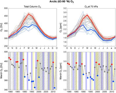
Figure 1 (Top panel) Seasonal cycle of polar cap averaged (63–90°N) total column and vertically-resolved ozone at 70 hPa from MERRA. The thin red/blue lines show the identified high/low ozone years and the thicker lines show the average of the high/low ozone years. (Bottom panels) Time series of total column and vertically-resolved at 70 hPa ozone from MERRA in March. Years identified as having high/low ozone abundances are indicated by red/blue circle markers. The hatching shows years when a major sudden stratospheric warming occurred; yellow shading indicates La Niña years and blue shading indicates El Niño years.
Download figure:
Standard image High-resolution imageStatistical significance between the subsets of data was evaluated using a Student's t statistic (as in Santer et al 2000) and are presented at the 95% confidence level based on a one-sided test. Pearson correlation coefficients are also calculated between linearly detrended March ozone and linearly detrended spring (March-April) surface temperatures and winds using monthly- or seasonal-mean data from 1979–2012. The statistical significance of the correlation coefficient was also evaluated using a Student's t statistic. Significant changes in daily maximum spring temperatures for selected regions are determined from probability distributions of daily GHCN station data. The distributions were estimated assuming a bin size of 20, estimated from the square root of the number of observations available in the selected set of years for Southern Asia (which had the most limited record); statistical significance was determined using a two-sample Kolmogorov-Smirnov test.
In this study, we chose March to represent spring Arctic ozone, which is the month with the largest observed ozone losses and is consistent with the constructed ozone forcings used in Smith and Polvani (2014). Calvo et al (2015) selected April as the indicator month; our analysis suggests that the observed maxima in ozone depletion peak one month earlier on average than in their model. We analyze the tropospheric response over March and April (hereafter referred to as spring). The tropospheric responses in March and April are fairly similar (discussed further in the results section). Therefore, we present the tropospheric responses in the spring average, to provide an improved signal to noise and for comparison with the earlier modeling studies.
Years with major sudden stratospheric warmings were identified using the climatologies from Charlton and Polvani (2007), for 1958–2002, and Kuttippurath and Nikulin (2012), for 2003–2012. Both studies use the criterion of zonal-mean zonal wind reversal from westerly to easterly at 60°N at 10 hPa to identify the onset of a major sudden stratospheric warming. Years with a strong influence from El Niño or La Niña were identified as when the National Weather Service Climate Prediction Center's Oceanic Niño Index (ONI) exceeded ±1 in any month from November through March (www.cpc.ncep.noaa.gov/products/analysis_monitoring/ensostuff/ensoyears.shtml). The ONI is calculated as the three month running mean of sea surface temperature anomalies from ERSSTv4 over the Niño-3.4 region (5°S–5°N, 120°W–170°W), where the anomalies are estimated from a 30-year period, which is updated every 5 years. The role of increasing well-mixed greenhouses gases was estimated as the difference between the years 2007–2012 and 1979–1984 (referred to below as 'historical').
3. Results
Figure 1 shows the seasonal cycle and interannual variability of total column and lower stratospheric (70 hPa) ozone from MERRA averaged over the Arctic. Years with low ozone anomalies in March are characterized by lower ozone abundances in early winter as well, and these anomalies persist throughout the summer. Figure 1 also shows time series of March total column and lower stratospheric ozone at 70 hPa with the ozone extremes (as defined in section 2.2) highlighted. Winters with major sudden stratospheric warmings and strong La Niña or El Niño events are also indicated. Low ozone anomalies predominate in the late 1990s. High ozone anomalies are observed in both the early 1980s as well as in the 2000s, which helps to distinguish the relationship of tropospheric climate with ozone from that of increasing well-mixed greenhouse gases.
Randel et al (2009) noted higher Northern Hemispheric polar ozone abundances during El Niño winters, as El Niño winters have a weaker polar vortex due to enhanced planetary wave activity (e.g. van Loon and Labitzke 1987). Iza and Calvo (2015) also found that the polar vortex was weaker in El Niño winters not only during canonical El Niño (Eastern Pacific El Niño) events but also during Central Pacific El Niño events coinciding with major sudden stratospheric warmings. In contrast, La Niña winters are characterized by a stronger vortex and negative ozone anomalies (Garfinkel and Hartmann 2007, Free and Seidel 2009). However, Butler and Polvani (2011) showed that the frequency of sudden stratospheric warming events was similar in El Niño and La Niña winters. As seen in figure 1, lower ozone abundances are overall observed in winters without a major sudden stratospheric warming, as compared to winters with them, while the relationship between extremes in Arctic spring ozone at 70 hPa and ENSO is less clear. This is consistent with Rieder et al (2013), who found that the fingerprint of ENSO on ozone was strongest in the tropics and mid-latitudes and diminished over the polar regions.
To illustrate the tropospheric impact of stratospheric ozone anomalies, figure 2 (leftmost column) presents the seasonal differences in polar cap (75–90°N) averaged ozone, temperature, and geopotential height, as well as zonal winds averaged over the North Atlantic (60 °W–0 °Eq) from 55–65 °N between years with low March ozone compared to high March ozone anomalies. Years characterized by low ozone anomalies in March show lower ozone throughout winter and into the fall in the lower stratosphere (left column of figure 2), as also seen in figure 1. Colder temperatures are also observed in late winter and persist through the fall in the lower stratosphere in years with low ozone.

Figure 2 Seasonal differences in polar cap averaged (75–90°N) ozone [%], temperature [K], and geopotential height [m] as well as North Atlantic (60°W–0°Eq) zonal winds [m s−1] averaged from 55–65°N from MERRA between years with low compared to high March ozone, years without major sudden stratospheric warmings as compared to years with them, winters with La Niña compared to El Niño events, and the historical time period (defined as 2007–2012 minus 1979–1984). Hatching denotes differences that are statistically significant at the 95% level.
Download figure:
Standard image High-resolution imageLower geopotential heights are observed in late winter and into the summer in the stratosphere in years with low ozone, consistent with the positive polarity of the NAM/NAO and corresponding to a stronger, colder polar vortex in the stratosphere and a poleward shift of the mid-latitude jet in the troposphere. Over the midlatitudes, years with low ozone anomalies show stronger North Atlantic zonal winds in winter and spring (bottom left panel of figure 2).
The additional columns of figure 2 show the behavior obtained in the same variables when different potential forcings are considered: years without major sudden stratospheric warmings compared to years with them; years with strong ENSO events, and the long-term change. Figure 2 shows that that the strongest and most robust differences in Arctic stratospheric and tropospheric winter and spring climate occur for the differences between years with low March ozone anomalies compared to high ozone anomalies. Differences in Arctic climate between years without major sudden stratospheric warmings and with them show similar patterns to the differences based on low and high March ozone, albeit weaker. This is not surprising as years with low/high March ozone anomalies tend to occur in winters without/with major sudden stratospheric warmings (figure 1). Figure S1 (available at stacks.iop.org/ERL/12/024004/mmedia) shows that the temperature changes obtained in figure 2 using MERRA are similar to those found using radiosonde station data from HadAT2, version 2 (Thorne et al 2005); therefore, these changes are not artifacts of the reanalysis.
Overall the stratospheric-tropospheric differences shown in figure 2 between La Niña and El Niño years are much weaker than those associated with interannual variability of ozone and the occurrence of major sudden stratospheric warmings. Note that Calvo et al (2011) found that only El Niño winters with SSWs have a robust impact on tropospheric climate through the stratosphere. The historical differences between the early 1980s and late 2010s in the Arctic stratospheric climate (right column of figure 2) show a weaker, warmer polar vortex in early winter, followed by a colder polar vortex in late spring, albeit weaker than in the analysis with ozone extremes. However, studies have shown that historical trends or differences in Arctic winter stratospheric climate are sensitive to the chosen end-year, suggesting that the historical responses are not robust to the chosen end-year (Manney et al 2005, Ivy et al 2014).
Figure 2 indicates that interannual variations of ozone in March project onto zonal-mean surface climate in spring. Figure S2 further explores the correlations between March ozone at 70 hPa with zonally-varying zonal wind at 500 hPa, sea level pressure, and surface temperatures in March, April, and the spring average (March and April). As seen in figure S2, there are regions with significant correlations between the Northern Hemisphere tropospheric climate and March ozone in both March and April individually, and the patterns exhibit several similar features in the two months, particularly in the surface temperature field (figure S2 bottom row). The tropospheric changes project onto the zonal-mean (figure 2) but also display strong zonal asymmetries (figure S2).
Figure 3 shows maps summarizing the regional differences in Northern Hemispheric tropospheric climate in spring between years with low and high ozone abundances in March. The figure is very similar to the right column of figure S2, but not identical since it is based on composite differences rather than correlations using March ozone (see also figure 4 in Smith and Polvani (2014) and figure 3 in Calvo et al (2015)). Figure S3 compares the results in figure 3 with the attendant results calculated for major sudden stratospheric warmings, ENSO, and the long-term trend. Years with low ozone are associated with a statistically significant poleward shift of the midlatitude jet over the North Atlantic (figure 3 top) that is similar to that noted in previous modeling studies (Smith and Polvani 2014, Calvo et al 2015). The differences in sea level pressure are consistent with the positive polarity of the NAM/NAO, with lower sea level pressures over the Arctic and higher pressures over the midlatitudes in spring for years with low ozone anomalies. The differences in spring surface temperatures show warmer temperatures over northern Siberia and southwestern Europe, and colder temperatures over southeastern Europe and southern Asia in years with low March ozone anomalies (figure 3).
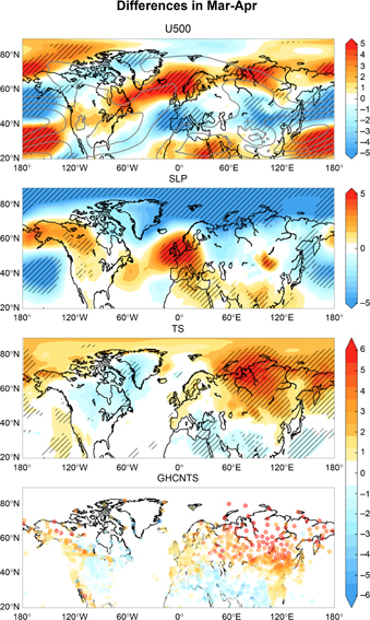
Figure 3 Differences (colors) in March-April zonal wind at 500 hPa [m s−1] and sea level pressure [hPa] from MERRA and surface temperatures [K] from ERA-Interim and GHCN for years with low March ozone compared to years with high March ozone. The contour lines show the climatological mean winds in the top panel; contours are every 5 m s−1 (..., −10, −5, 5, 10,...). Hatching denotes differences that are statistically significant at the 95% level.
Download figure:
Standard image High-resolution image
Figure 4 (Top panel) Correlation coefficients of linearly detrended March Arctic (63–90°N) ozone at 70 hPa compared to (colors) linearly detrended March-April surface temperatures and (vectors) winds at 925 hPa from ERA-Interim, where the correlations were calculated for both the zonal and meridional winds and are represented as a vector, the vector scale is indicated in the top right; the green contours enclose areas that are statistically significant at the 95% level. (Middle and bottom panels) Time series of linearly detrended March Arctic (63–90°N) ozone at 70 hPa (black lines) and March-April surface temperatures (pink or blue lines) from ERA-Interim at selected latitudes and longitudes (shown as stars on the top panel); the y-axis for surface temperatures with blue lines has been inverted for clarity.
Download figure:
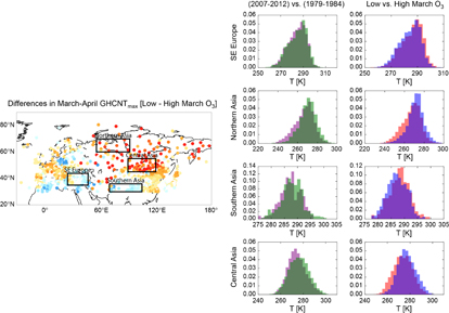
Standard image High-resolution imageTo highlight the relationships between March ozone and spring surface temperatures on interannual timescales, figure 4 shows the correlation coefficients of March Arctic ozone at 70 hPa with spring averaged surface temperatures and near-surface winds from ERA-Interim. The temperature results are similar to those in the composite difference analysis of figure 3 and identical to those in correlation analysis in the right column of figure S2. Over southeastern Europe and southern Asia, years with low ozone anomalies tend to have colder surface temperatures, as seen by the positive correlations. Over northern Asia, low ozone anomalies are associated with warmer surface temperatures, corresponding to southwesterly winds bringing warmer air poleward (as seen in the wind vectors in figure 4). Overall, more areas are statistically significant than in the composite analysis due to the inclusion of more years in the analysis. The associated time series of surface temperatures for selected locations are shown in figure 4 (middle and bottom panels) and illustrate locally strong relationships with March Arctic spring ozone, with correlations of 0.46 for Grand Rapids, MI, USA, −0.67 for eastern Siberia, −0.77 for central Russia, and 0.67 for Nepal; all are statistically significant at the 95% level.
To investigate the possible relationship between spring ozone and daily surface temperature extremes, figure 5 shows the probability distributions for daily maximum temperatures in spring for selected regions displaying high correlation coefficients between March ozone and linearly detrended spring surface temperatures (figure 4). The distributions of daily maximum temperature between the high and low ozone years in the regions shown in figure 5 were all statistically different at the 95% level based on a two-sample Kolmogorov-Smirnov test. Figure 5 (right) also shows that some of the regions show strong differences in the historical time period, as would be expected from increasing well-mixed greenhouse gases (as also seen in figure S3). Over southeastern Europe and southern Asia, years with low ozone anomalies display colder extreme spring temperatures that appear to be more extreme than those in the historical time period. Over Siberia and central Asia, years characterized by low ozone show warmer temperatures than years with high ozone, but also reveal substantial changes in the historical time period. Thus, figure 5 suggests that the connection between stratospheric ozone changes on extreme surface temperature may be comparable to those associated with increasing GHGs over certain regions.
Figure 5 (Left panel) Differences in March–April monthly-mean surface temperature data from GHCN for years with low March ozone compared to years with high March ozone. The boxes indicate the regions over which the probability distributions were calculated. (Right panels) Probability distributions of daily maximum surface temperatures in March–April from GHCN for historical late period (2007–2012; green) compared to the early period (1979–1984; purple) and for years with low spring ozone (blue) compared to years with high spring ozone (red).
Download figure:
Standard image High-resolution image
4. Conclusions
Previous studies (Baldwin and Dunkerton 2001, Thompson and Wallace 2001) have shown direct coupling between the stratospheric and tropospheric circulations in NH winter. Our analysis illustrates the value of ozone measurements as an indicator for stratospheric circulation change, and shows that the tropospheric anomalies persist after the extreme ozone anomalies for up to one month. Springs characterized by low ozone anomalies in March show a stronger, colder polar vortex in the stratosphere in late winter and early spring. In the troposphere, years with negative ozone anomalies during March are associated with circulation anomalies consistent with the positive polarity of the NAM/NAO that persist into April, including a poleward shift of the North Atlantic jet, lower than normal temperatures over eastern North America, southeastern Europe, and southern Asia, and higher than normal temperatures over northern and central Asia. Furthermore, we suggest that these stratospheric-tropospheric coupled results in spring are most pronounced when analyzed in the context of Arctic ozone extremes, and generally less apparent when analyzed for ENSO events or increasing greenhouse gases.
Our analysis of several observational datasets supports a linkage between March Arctic lower stratospheric ozone and spring Northern Hemispheric extratropical surface climate. Although there is a limited number of extreme ozone years available for analysis, broad agreement between the observations and modeling results gives confidence in our findings (Calvo et al 2015). Further, correlations between March stratospheric ozone and surface temperatures averaged for March and April are significant in certain locations even when all years are considered (figure 4). Finally, while it is clear that tropospheric greenhouse gas increases have driven many changes in surface climate extremes in recent decades, this study suggests that stratospheric extremes are significant contributors to extreme surface temperatures in spring at some locations (figure 5). While the linkages between ozone and surface climate highlighted here do not necessarily imply causality, our results do indicate predictability of March ozone for spring tropospheric climate, particularly in certain regions. Future work is needed to evaluate the predictive skill of using ozone for Northern Hemispheric tropospheric climate.
Acknowledgments
We thank two anonymous reviewers for their helpful comments and suggestions. DJI and SS were supported by National Science Foundation (NSF) Atmospheric Chemistry grant AGS-1539972. NC acknowledges partial support from the Spanish Ministry of Economy and Competitiveness through the PALEOSTRAT project (CGL2015-69699) project and the European Project 603557-STRATOCLIM under program FP7-ENV.2013.6.1-2. DWJT is supported by the NSF Climate Dynamics Program.