
Abstract
The impacts of historical droughts and heat-waves on ecosystems are often considered indicative of future global warming impacts, under the assumption that water stress sets in above a fixed high temperature threshold. Historical and future (RCP8.5) Earth system model (ESM) climate projections were analyzed in this study to illustrate changes in the temperatures for onset of water stress under global warming. The ESMs examined here predict sharp declines in gross primary production (GPP) at warm temperature extremes in historical climates, similar to the observed correlations between GPP and temperature during historical heat-waves and droughts. However, soil moisture increases at the warm end of the temperature range, and the temperature at which soil moisture declines with temperature shifts to a higher temperature. The temperature for onset of water stress thus increases under global warming and is associated with a shift in the temperature for maximum GPP to warmer temperatures. Despite the shift in this local temperature optimum, the impacts of warm extremes on GPP are approximately invariant when extremes are defined relative to the optimal temperature within each climate period. The GPP sensitivity to these relative temperature extremes therefore remains similar between future and present climates, suggesting that the heat- and drought-induced GPP reductions seen recently can be expected to be similar in the future, and may be underestimates of future impacts given model projections of increased frequency and persistence of heat-waves and droughts. The local temperature optimum can be understood as the temperature at which the combination of water stress and light limitations is minimized, and this concept gives insights into how GPP responds to climate extremes in both historical and future climate periods. Both cold (temperature and light-limited) and warm (water-limited) relative temperature extremes become more persistent in future climate projections, and the time taken to return to locally optimal climates for GPP following climate extremes increases by more than 25% over many land regions.
Export citation and abstract BibTeX RIS

Content from this work may be used under the terms of the Creative Commons Attribution 3.0 licence. Any further distribution of this work must maintain attribution to the author(s) and the title of the work, journal citation and DOI.
1. Introduction
The past two decades have seen extremely warm temperatures relative to historical averages (Hansen et al 2010, 2012). These warm temperature extremes and associated droughts significantly reduced ecosystem carbon uptake on several continents, as estimated by a combination of process models, surface CO2 flux measurements, and vegetation remote sensing (Ciais et al 2005, Zhao and Running 2010, Schwalm et al 2012, Reichstein et al 2013). Such trends raise concerns of diminished carbon uptake in response to global warming (Phillips et al 2009, Zhao and Running 2010, Allen et al 2010, Saatchi et al 2013, Reichstein et al 2013), which would support feedbacks that accelerate global warming by leaving more CO2 in the atmosphere and less in soils and vegetation (Friedlingstein et al 2006, Arora et al 2013). Furthermore, observed sharp declines in ecosystem carbon uptake with increasing temperature suggest that land ecosystems already operate near high temperature thresholds (Doughty and Goulden 2008, Zhao and Running 2010, Corlett 2011). These observations motivate ecological impact assessments using historical warm temperature extremes as analogs of global warming (Williams et al 2007, Beaumont et al 2011), giving the impression of ecological tipping-points above historical temperature bounds (Mora et al 2013). It is therefore important to determine if the observed decline of ecosystem carbon uptake with increasing temperature in the historical record is indicative of a fixed threshold temperature for declining ecosystem productivity, and if the reduction in ecosystem carbon uptake in response to recent heat-waves and droughts thereby signals a turning point toward diminished ecosystem carbon uptake under global warming.
The historical record provides ample evidence that land carbon uptake declines under warm temperature extremes (Doughty and Goulden 2008, Zhao and Running 2010, Corlett 2011, Saatchi et al 2013), but it is not clear whether these historical events are indicative of global warming impacts on ecosystems. Here we are concerned with potential changes in precipitation and soil moisture under global warming that would make historical warm temperature extremes poor analogs of global warming. For example, heat-waves typically occur under 'blocking' high pressure weather systems that carry subsiding dry air thermodynamically unfavorable for precipitation (Black et al 2004, Girardin et al 2006, Pezza et al 2012). These weather systems can lead to droughts by suppressing precipitation, and through soil-temperature feedbacks that warm and dry soils (Koster et al 2009, Seneviratne et al 2010, Sheffield et al 2012). Although extreme temperatures characteristic of historical heat-waves are projected to increase in frequency and persistence under global warming (Kharin et al 2013, Sillmann et al 2013), these increases arise mostly from increases in average temperatures as opposed to increases in temperature variability (Rhines and Huybers 2013). Warm temperature extremes in historical records are tied to processes giving rise to temperature variability, whereas increases in average temperatures are associated with radiative forcing by long-lived greenhouse gases in future climate projections. These different processes can have different impacts on precipitation and soil moisture, and these differences lead to different impacts on ecosystem carbon uptake, as shown here. The potential for acclimation and adaptation of plants to global warming is an additional potential difficulty with historical analogs that is not considered here, as these effects are not included in current Earth system models (ESMs), and may be limited in effectiveness to species already endemic to Earthʼs warmest climates (Berry and Bjorkman 1980).
For reasons further discussed here, we distinguish between temperature departures from historical averages and temperature variability defined by departures from averages within a given climate period, which may be historical or from an ESM future climate projection. In addition to increasing surface temperatures, the radiative forcing by well-mixed greenhouse gases also increases vertically-integrated tropospheric radiative cooling, which supports higher globally-averaged precipitation rates (Held and Soden 2006), and these precipitation increases could partially offset the soil moisture losses at higher temperatures. Additionally, increased atmospheric CO2 concentrations can increase plant water-use efficiency, meaning a given rate of photosynthesis can be maintained with less transpiration (Sellers et al 1996), which could allow net carbon uptake to occur in drier climates that would otherwise induce water stress.
Moreover, the precipitation rate is not a fixed function of temperature, and this non-stationarity in the joint probability distribution of temperature and precipitation could significantly affect the relationship between temperature and soil moisture in future climate projections. For example, moist convection is a significant if not dominant source of precipitation over much of the tropics and over the growing season in mid-latitudes (Schumacher and Houze 2003, Yang and Smith 2008), and trigger surface temperatures for moist convection increase along with tropospheric average temperatures in global climate models and in observations (Williams et al 2009, Johnson and Xie 2010). As discussed in the latter studies over the tropical oceans, the onset of convective precipitation should occur at higher surface temperatures under global warming, both because the whole troposphere warms under increased radiative forcing by well-mixed greenhouse gases, and because moist convective instability requires warm near-surface air relative to the overlying free-troposphere. This shift in precipitation onset to warmer surface temperatures could potentially mitigate the drying effects of warm temperature extremes, but would be limited by the availability of water vapor over land.
In this study we examine changes in precipitation, soil moisture, and ecosystem carbon uptake, to evaluate the usefulness of historical warm temperature extremes as analogs of global warming impacts on ecosystem carbon uptake, using ESMs that represent the coupled carbon–climate system. These ESMs include the relevant radiative and thermodynamic processes needed to distinguish between historical warm temperature extremes and global warming in terms of their impacts on ecosystem productivity.
Absolute temperature distributions
We analyzed gross and net primary production (GPP and NPP) in nine ESMs (see supplemental table S1) used in the coupled model inter-comparison project (CMIP5, experiments esmHistorical and esmrcp85; (Taylor et al 2012)). As discussed above, temperatures that are extreme relative to historical averages could have different impacts on photosynthesis under global warming, particularly if changes in precipitation and soil moisture coincide with global warming. We illustrate this non-stationarity of climate impacts on ecosystems by examining how GPP is distributed as a function of surface temperature (near surface temperarature), and how this distribution changes between historical and future (RCP8.5) climate projections. The temperature distributions of GPP reveal the temperatures most and least favorable for photosynthesis.
The distributions were estimated from monthly-averaged ESM output by finding all values of GPP that coincided with temperatures falling within approximately 1 °C bins, using data at each model grid cell separated into five different ecosystem types (conifer, tropical, and mixed forests, fields/woods/savanna, and crops; see the supplemental materials for ecosystem definitions and spatial distributions). These analyses were performed only for the growing season defined by the five months of the year having highest GPP on average (calculated for historical and RCP8.5 climates separately, at each grid cell of each model). The averaging of GPP within temperature bins was performed separately for each ecosystem type, resulting in a single distribution function for each ESM and ecosystem type. The distributions were then averaged over the nine ESMs, resulting in one ensemble average distribution for each ecosystem type (figure 1, row A). Also shown are the temperature distributions of soil moisture and precipitation (figure 1, rows B and C), which were estimated using the same methods as for GPP. Fractional soil moisture was calculated as the mass of water in the upper soil layer in each model normalized by its maximum value. Both historical and future climates were searched for a single maximum soil moisture value at each grid cell, using monthly model output. The probability of each temperature bin is also shown (figure 1, row D).

Figure 1. Panel A: Ensemble-averaged temperature distributions of GPP, obtained by averaging GPP within temperature bins of approximately 1 °C (error bars indicate the standard error of the ensemble average). Future (2070–2100) and historical (1970–2000) climates are shown in red and blue, respectively. Panel B: As in (A), but for fractional soil moisture (soil moisture content in the upper model layer normalized by its maximum). Panel C: As in (A), but for precipitation in units of latent heat flux. Panel D: Probability density function (PDF) estimated from the number of months and grid points within each temperature bin, averaged over the CMIP5 ensemble (the area under each PDF sums to unity). All results are for the growing season only.
Download figure:
Standard image High-resolution imageThere are overall increases in GPP mostly above 280 K in future RCP8.5 (2070–2100) climates (figure 1, row A, red lines) relative to historical (1970–2000) climates (figure 1, row A, blue lines), consistent with CO2 fertilization effects noted previously (Friedlingstein et al 2006). There are also sharp declines in GPP at high temperature extremes in the historical climates, similar to the observed declines in GPP with warm temperature extremes discussed in the introduction. However, the declines in GPP set in at higher temperatures in RCP8.5 climates, closely tracking the increases in temperature thresholds for declining soil moisture (figure 1, row B) and precipitation (figure 1, row C). In contrast to the significant changes in temperature distributions of GPP at warm temperatures, at cold temperature extremes GPP is almost constant between RCP8.5 and historical climates, suggesting an intrinsic cold temperature limitation to GPP in these ESMs (figure 1, row A). Additional analyses confirm that the broad enhancement of GPP at high temperatures is a result of CO2 fertilization (see supplemental materials figure S 2), and that the shift in the temperature for onset of GPP decline to warmer temperatures is not simply due to elevated CO2. These additional analyses were performed on the esmFdbk1 experiment, in which the carbon cycle 'sees' a fixed CO2 concentration, but the radiation (and hence climate) sees a 1% per year rise in CO2.

Figure 2. Top row: Ensemble-averaged change in gross primary production (GPP) averaged over all temperatures (a), and over temperatures greater than the 90th percentile of historical (b), during the growing season. Bottom row: Ensemble-averaged change in net biosphere production (NBP) averaged over all temperatures (c), and over temperatures greater than the 90th percentile of historical (d), during the growing season. Changes are defined as future (2070–2100) minus historical (1970–2000) values. Stippling indicates where at least 7 of the 9 ESMs agree on the sign of the change.
Download figure:
Standard image High-resolution imageThe above results caution against using metrics of climate stresses on ecosystems that are based on departures of projected future temperatures from historical temperature bounds, and suggest that the observed declines in GPP associated with historical warm temperature extremes are correlations that arise from the separate dependence of GPP on soil moisture, and from the correlation of soil moisture with temperature. The relationship between soil moisture and temperature is more complicated than these correlations would suggest, as evidenced by the shift in maximum soil moisture to warmer temperatures under global warming. These changes in soil moisture can be understood by the similar shift in maximum precipitation to warmer temperatures along with the shift in the whole temperature probability density function (cf figure 1 rows C, D). These results are consistent with the onset of moist convection occurring at warmer temperatures under global warming, as discussed above. As evidence of an increase in convective trigger temperature, we note that the distribution of boundary layer buoyancy, a precursor to deep convection, shifts to warmer temperatures (see supplemental materials figure S 3). Thus, as average temperatures increase under global warming, the occurrence of maximum precipitation shifts to warmer temperatures along with the average temperature, thereby increasing soil moisture and GPP at warm temperature extremes historically associated with drought. In tandem with this shift in maximum precipitation, the onset of low soil moisture characteristic of droughts (figure 1, panel B) also shifts to warmer temperatures.
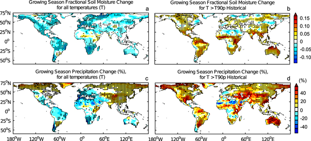
Figure 3. Top row: Ensemble-averaged change in fractional soil moisture averaged over all temperatures (a), and averaged over temperatures greater than the 90th percentile of historical (b), during the growing season. Bottom row: Ensemble-averaged change in precipitation averaged over all temperatures (c), and over temperatures greater than the 90th percentile of historical (d), during the growing season. Changes are defined as future (2070–2100) minus historical (1970–2000) values, expressed as a percentage of historical values for precipitation. Stippling indicates where at least 7 of the 9 ESMs agree on the sign of the change.
Download figure:
Standard image High-resolution imageTo ensure our results are not sensitive to averaging over the broadly defined ecosystem types, we further examined the spatial distribution of growing season changes in GPP, precipitation, and soil moisture between future and historical climates (figure 2). We also examined whether results for GPP are relevant to the net carbon balance of the biosphere by examining net biosphere production (NBP), defined as the balance of NPP and carbon losses due to heterotrophic respiration, fire, and harvested biomass. Changes in GPP were averaged over all temperatures (figure 2(a)), and over temperatures greater than the 90th percentile of historical temperatures (figure 2(b), labeled  historical temperatures). In almost all mid-latitude and tropical land regions, the increase in GPP at warm temperature extremes (T
  T90p historical temperatures) is larger than the increase in GPP averaged over all temperatures, which is the same overall result obtained from the individual temperature distributions of GPP shown in figure 1. Exceptions are over portions of the Pacific coast of North America, Central Asia, and the Arctic, where the average increase in GPP is slightly larger than the average over warm temperature extremes. We obtained similar results for NBP as for GPP, in that changes in NBP between future and historical climates are in most cases larger at warm temperature extremes (
 historical; figure 2(d)) than when averaged over all temperatures (figure 2(c)).
Spatial distributions of soil moisture (figure 3) also reveal significant differences between changes in average soil moisture and changes in soil moisture at warm temperature extremes. It is clear from these spatial distributions that our results showing large increases in soil moisture at warm temperature extremes (figure 1, panel B) are not in disagreement with previous studies showing a decline in soil moisture with global warming (Sheffield and Wood 2008, Wehner et al 2011, Schwalm et al 2012), because those studies did not examine how the changes in soil moisture are distributed over temperature. When averaged over all temperatures, there is a significant decline in soil moisture over many land regions (figure 3(a)). However, there is a significant increase in soil moisture at temperatures greater than the 90th percentile of historical temperatures (figure 3(b)). This increase in soil moisture at warm extremes is a result of increased precipitation at warm extremes, and not a reduction in evaporation (see supplementary figure S 4). These findings are consistent with shifts in the distributions of soil moisture to warmer temperatures shown in figure 1 (panel B), and help to explain why the warm temperature thresholds for GPP decline occur at higher temperatures in future climate projections than in historical climates. Spatial distributions of precipitation changes (figures 3(c), (d)) are broadly similar to those of soil moisture changes, particularly at warm temperature extremes (figure 3(d)) where there is an increase in both precipitation and soil moisture over many land regions. The correlation between changes in soil moisture and changes in precipitation is less clear when averaged over all temperatures, particularly at high latitudes (figure 3(c)). These results further demonstrate that historical relationships between GPP and warm temperature extremes are not suitable indicators of the impacts of global warming on GPP, because precipitation and soil moisture are not uniquely related to temperature.

Figure 4. GPP (panel A), fractional soil moisture (panel B), and downwelling solar radiation (panel C), distributed as functions of relative temperature (T
 ). Panel D: Logarithmic derivatives of (minus) soil moisture and canopy absorbed solar radiation with respect to temperature, expressed as a percentage change per K, where the intersection of these two curves is the location of a local minimum or maximum in GPP (see equation (2)). Thick lines indicate where the statistical significance of the difference between historical (blue) and future (red) simulations exceeds the 90% confidence level. All results are for the growing season only.
Download figure:
Standard image High-resolution imageRelative temperature distributions
We have shown that the departure of temperature from historical temperature bounds is a poor metric of the impacts of climate extremes on ecosystem carbon uptake, in terms of both GPP and NBP. Here we define an improved metric for use in comparing historical and future climate projections, using the departure of temperature from a locally optimal temperature for GPP (hereafter referred to as relative temperature, or T
 ), where our use of the term 'local' refers to the dependence of this maximum on a particular climate period (historical or future). This relative temperature is defined as T
 = T−T
= T−T
 , where T is monthly average near-surface air temperature, and T
 is the temperature at which GPP has a maximum within a given climate period. Results were similar when defining T
 based on the average of temperatures over which the highest 10% of GPP occurs (not shown). We estimated T
 for each model grid cell and for each month of the growing season. For example, T* for July is the temperature corresponding to the highest GPP of all 30 Julys between years 1970 and 2000 (for historical). Distributions of GPP, soil moisture, and downwelling solar radiation were estimated in terms of T
 (figure 4), using the same method described above for absolute temperature.
By design of the metric, maximum GPP occurs when T' = 0 (figure 4, panel A), for both historical and future climate projections. Moreover, sensitivities of GPP to relative temperatures are similar between future and historical climates (i.e. GPP declines away from T
 in both future and historical climates), which indicates that the impacts of T
 extremes on GPP are approximately invariant with average climate. This similarity in impacts regardless of the climate period makes T
 an improvement over absolute temperature as a measure of climate extremes. We also note that the impact of temperature extremes on productivity in the ESMs is similar to observations, for example the approximately 30% reduction in GPP with a positive 2 K relative temperature in ESM historical crop systems (figure 3, panel 5A) is in agreement with observational estimates during the 2003 heat-wave and drought in Europe Ciais et al 2005. The onset of water stress (i.e. low soil moisture) at high relative temperatures is consistent with the results of observational studies demonstrating a dryness control on CO2 uptake that sets in at relatively high temperatures (Yi et al 2010).
We similarly estimated the relative temperature distributions of soil moisture and surface downwelling solar radiation (figure 4, panels B, and C, respectively), which we used to diagnose the factors contributing to the temperature of locally maximum GPP and its increase under global warming. The processes that determine the temperature of maximum GPP can be inferred using a simplified GPP diagnostic (Betts et al 2004), given by

where APAR is the incident photosynthetically active radiation absorbed by leaves, ε is a potential light-use efficiency parameter (i.e. light-use efficiency in the absence of environmental stress),  is a factor accounting for water stress due to soil moisture, and
  accounts for the sensitivity of photosynthesis to temperature through enzyme kinetics. APAR was estimated from predicted leaf area index (LAI) assuming a constant light extinction coefficient, e.g. as in (Betts et al 2004). The change in LAI between future and historical climates taken into account through LAI in the exponential term in the Beer–Lambert equation. Although water stress and enzymatic controls on photosynthesis and their coupling to climate are represented in the latest generation of ESMs analyzed here, (e.g. Sellers et al 1996), these terms are not model output variables. The temperature stress factor was therefore diagnosed separately using a quadratic function of temperature (Betts et al 2004). Water stress (
 ) is often characterized as a nonlinear function of soil moisture content (Seneviratne et al 2010), but we used a linear fit as quadratic or higher-order functions of soil moisture did not change our results for the location of maximum GPP with respect to temperature.
We found that the temperature of GPP maximum in the ESMs can be diagnosed as the temperature at which the combination of water stress and light limitations is minimized, assuming constant light-use efficiency. This minimum can be quantified by taking the logarithm and differentiating equation (1) with respect to temperature
The maximum in GPP occurs where the left hand side of equation (2) is zero. We neglected the direct temperature sensitivity through enzyme kinetics ( ), as we found it to be much smaller than the water and light sensitivities for temperatures near to the temperature at maximum GPP. Thus, the temperature at maximum GPP was determined by the intersection of the temperature derivative of the APAR term (solid lines in figure 4, panel D) with the (negative) temperature derivative of the water stress term (dashed lines in figure 4, panel D).
The intersection of these derivatives is indeed very close to T
 (figure 4, panel D), meaning that a local maximum in GPP occurs at temperatures that minimize the combination of water stress and light limitations on GPP. The location of the intersection of these derivatives in T
 does not significantly change between the future (red lines in figure 4, panel D) and historical climates (blue lines in figure 4, panel D), which indicates that water stress and light limitations are fundamental processes controlling GPP that are not specific to particular climates in these ESMs. Furthermore, the T
 metric is a useful measure of these processes. Note that the intersection occurs for non-zero values of the APAR and water stress term derivatives, meaning that the temperature of maximum GPP is not simply the temperature of maximum soil moisture or of maximum downwelling solar radiation separately, but a combination of both factors. The decrease in downward solar radiation at low values of T
 is not due to seasonality, since T
 and T
and T
 are estimated separately for each month. Negative T
 values are accompanied by cloud cover, as diagnosed by cloud radiative effects on the surface energy balance (not shown).
The sensitivity of photosynthesis to cold temperature extremes is also similar between historical and future climates, as seen by comparing the slopes of the GPP-T
 curves between historical and future climates for negative T
 . This result may be surprising considering that the coldest growing season temperatures increase with global warming. However, the decline in GPP with cold temperature extremes (negative T
 values) is likely not an intrinsic response to temperature but rather a result of cloudy and therefore light-limited and relatively cool conditions, with reduced downward solar radiation relative to warmer temperatures (figure 4, panel C). Note that we have not considered impacts of changes in snowfall or length of growing season, which are additional factors in high-latitude climates. From an ecological point of view, there are also stresses that depend on absolute temperature that we have not considered, such as the minimum winter temperatures necessary for eliminating mountain pine beetle populations. Such examples serve as a reminder that it is difficult to define a single climate measure that encompasses the full range of ecological responses to climate. Here we focus on the impacts of climate extremes on photosynthesis, for which T
 is a useful metric.
Changes in the temperature at maximum GPP closely track changes in the growing season average temperature between historical and future climate projections (figure 5). This result was not anticipated a priori, and suggests that a simplified relative temperature metric could be defined as the departure of temperatures from an average within a particular climate period. The close correspondence of the average growing season temperature with the temperature at maximum GPP is related to the strong dependence of GPP on soil moisture, which has a local maximum near to the peak in the probability density function of relative temperature (cf figure 4, row B and figure 6, row A). In fact, the peak in the probability density function (figure 6, row A) is located near  , which is the relative temperature for both maximum soil moisture and GPP. These results are suggestive of strong land–atmosphere coupling in these ESMs, although determining the existence and direction of this coupling (and possible feedbacks) is beyond the scope of our present study. It is also apparent that the temperature at maximum GPP is slightly higher than the growing season average temperature for most ecosystems (figure 5), which is likely a result of the dual constraints of soil moisture and light on GPP, with light limitations on GPP being associated with cloud cover and negative relative temperatures (e.g. Figure 4, row C).

Figure 5. Temperature at GPP maximum as a function of the growing season average temperature, for each ecosystem type. Lengths of crosshairs indicate the standard error of the CMIP5 ensemble average. Both future and historical averages are shown and are connected by a straight line for each ecosystem type (the temperature of GPP maximum increases monotonically with growing season average temperature between future and historical simulations.) The black line indicates a 1 : 1 scaling.
Download figure:
Standard image High-resolution image
Figure 6. Panel A: Logarithmic probability density function of T
 , log(PDF). Panel B: Average change in temperature following the occurrence of each T
 value, during the growing season. Thick lines indicate where the statistical significance of the difference between historical (blue) and future (red) simulations exceeds the 90% confidence level. Monthly temperature changes were seasonally de-trended by subtracting the monthly climatology.
Download figure:
Standard image High-resolution imageImpact of increased relative temperature variance on GPP
There is an increase in the probabilities of extreme relative temperatures under global warming as evidenced by the widening of probability density functions of relative temperature (figure 6, row A), plotted on logarithmic y-axes to emphasize the tails of the distributions. This pattern implies an increase in occurrence of climate extremes that are relatively unfavorable for GPP under global warming. Here we quantify the impact of this increase in probability of T
 extremes on GPP. Changes in average GPP between historical and future climate projections (hereafter
  ) were decomposed into components due to (1) the change in probability of each relative temperature, and (2) the response of GPP to CO2 and climate change at a given relative temperature. These terms were estimated according to
The first right-hand side term is the contribution due to the change in probability (P) of relative temperature extremes (i.e. widening of the distributions with global warming) holding GPP constant at its historical value, the second term is the contribution due to changes in GPP within each T
 bin holding the probability of each bin constant, and the third term is the covariance of both changes. Similar methods have been used previously to examine changes in atmospheric variables in response to a warming climate (Bony et al 2004). Note that higher probabilities of relative temperature extremes can impact GPP both because GPP is lower at these extremes, and because higher probabilities of extremes necessarily imply lower probabilities of favorable climates for GPP (i.e. lower probabilities near T
 ). Our method accounts for these effects through the first right-hand side term of equation (3).
We focus on the first right-hand side term of equation (3) (results for the other terms are not shown), from which we infer that the increase in probability of relative temperature extremes in future climate projections acts to reduce GPP by 0.2–1.4% per K of future warming (supplemental table S2), depending on the ecosystem type. This result varied by model (supplemental table S3) from 0.19 to 1.8% per K. Note that we divided the whole expression (equation (3)) by the change in average temperature between the two 30 year climate periods (i.e. difference in temperature averages between the periods 2070–2100 and 1970–2000) to express results in units per K of warming.
Increase in persistence of climate extremes
Further implications of increased probabilities of relative temperature extremes are investigated here in terms of the persistence of these extremes. Increased persistence of warm extremes could potentially place greater stresses on ecosystems than if these extremes were more frequent but of short duration. We estimated the rate of return to T
 following each non-zero value of T
 , using time derivatives of temperature calculated from the change in temperatures (hereafter
  ) between the initial month of each extreme and the month following each extreme. In calculating
  , we used seasonally de-trended temperatures to separate average seasonal temperature variations from temperature changes in response to extremes. The temperature change (
 ) is shown in figure 6 (panel B), where it is clear that there are significant declines in magnitudes of warming following the occurrence of T
 and declines in magnitudes of cooling following the occurrence of T
 . A time-scale for return to T
 was then estimated from T
 , where
  is one month. Note that this time-scale is estimated from a rate that is assumed constant over the lifetime of each extreme event. From these estimates, we determined that the time taken to recover from cold relative temperature extremes increases under global warming (figure 7(a)), particularly over much of the tropics, indicating an increase in persistence of light-limited regimes under global warming. An increase in persistence of light-limited conditions does not necessarily imply an overall increase in cloud cover, but rather that there is an increase in the relative frequency of climates having a combination of high soil moisture and low values of downwelling solar radiation with respect to the requirements for maximum GPP. There is also a significant increase in persistence of warm relative temperature extremes by about 25% (figure 7(b)), especially over North America, Europe, and Asia. This 25% increase translates into an increase in total duration of warm relative temperature extremes by about 2.5 weeks on average, for a typical life-time of about 1.75 months (average life-times of cold and warm extremes are shown in figure 7(c), (d), respectively) including the one month during which the initial extreme occurs.

Figure 7. Top panel: Changes in warming rates following cold relative temperature extremes (a), and changes in cooling rates following warm relative temperature extremes (b), where changes are defined as differences between historical and future climate projections (future minus historical) and expressed as percentages of historical rates. Bottom panel: Average lifetime of cold relative temperature extremes (c), and average lifetime of warm relative temperature extremes (d), in historical climates, as estimated by monthly changes in relative temperature. Stippling indicates where at least 7 of the 9 ESMs agree on the sign of the change. All results are for the growing season only.
Download figure:
Standard image High-resolution image
Conclusions
The ESMs examined here predict sharp declines in GPP at warm temperature extremes in historical climates, similar to the observed correlations between GPP and temperature during historical heat-waves and droughts. However, these declines in GPP set in at higher temperatures under global warming. Similarly, there is also an increase in the temperature beyond which soil moisture and precipitation decline at warm temperature extremes. Based on these results, we conclude that temperatures that are extreme relative to historical averages have different impacts on photosynthesis under global warming, because of changes in precipitation and soil moisture that accompany the warming induced by increases in CO2 concentrations. Although average growing season soil moisture significantly declines under global warming over most land regions, both precipitation and soil moisture increase at warm temperature extremes currently associated with precipitation and soil moisture minima. These results suggest that the observed declines in GPP associated with historical warm temperature extremes are correlations that arise from the separate dependence of GPP on soil moisture, and from the correlation of soil moisture with temperature. The correlation of soil moisture with temperature is not constant under climate change, and this change should be taken into account when inferring future extreme climate impacts from present-day observations. Our results pertain to assumed fixed temperature thresholds for onset of water stress and do not preclude the existence of other absolute temperature thresholds.
Observational studies can account for non-stationarity in the relationship between GPP and temperature by examining the sensitivity of GPP to temperature anomalies defined relative to a local temperature optimum for GPP. This sensitivity remains similar between future and historical or present-day climates, which makes relative temperature an improvement over absolute temperature as a measure of climate extremes for comparing historical and future climate projections. The models show little interaction between the sensitivity of GPP to temperature anomalies and the trend in GPP with rising CO2. Hence, observed declines in present-day GPP with heat and drought extremes may be representative of similar declines in the future caused by such temperature variability, when temperature extremes are defined by temperature relative to a local temperature optimum for GPP. Furthermore, the models indicate that temperature variability may increase and drought events may be more persistent in the future, such that the net reduction in GPP due to climate extremes may be greater in the future when accounting for both the probability and impact of these extremes. We estimated a reduction in GPP of up to 1.4% per K of warming in ESM projections due to an increase in occurrence of climate extremes under global warming.
This study provides several new targets for observations of the carbon cycle in a changing climate. The concept of relative temperature leads to insights into how GPP responds to climate extremes under global warming. We found that GPP has a local maximum at a temperature that minimizes the combination of water stress and light limitation. This local maximum is an important outcome of the CMIP5 ESMs because it is robust across ecosystem types, has an interpretation in terms of the processes controlling GPP, and can be tested using observations. The concept of diagnosing climate influences as a departure of GPP from an optimum has been applied previously to interpret observational flux data from FLUXNET (Yi et al 2012), and suggests a model-observation comparison strategy. Our results also indicate that the reduction in GPP due to climate extremes under global warming results from an increase in the persistence of climates that are extreme relative to the requirements for optimal photosynthesis. This finding calls for observational studies aimed at detecting trends in the persistence of climate extremes and trends in the length of time for recovery of ecosystem carbon uptake following extreme events. Additionally, the predicted linear relationship between changes in the temperature at local maximum GPP and changes in the average growing season temperature is a robust emergent result from these ESMs, and an important target for carbon cycle observations. Observations combined with the analyses presented here will be useful in evaluating and further developing ESM representations of ecosystem carbon uptake, for predicting climate change impacts on ecosystems.
Acknowledgments
This research was supported by the Director, Office of Science, Office of Biological and Environmental Research of the US Department of Energy under Contract No. DE-AC02-05CH11231 as part of the Atmospheric System Research and Regional and Global Climate Modeling (RGCM) Programs. We acknowledge the World Climate Research Programmeʼs Working Group on Coupled Modelling, which is responsible for CMIP, and we thank the climate modeling groups (listed in table S1 of this paper) for producing and making available their model output. For CMIP the US Department of Energyʼs Program for Climate Model Diagnosis and Intercomparison provides coordinating support and led development of software infrastructure in partnership with the Global Organization for Earth System Science Portals.