

Abstract
An ensemble approach is used to examine the sensitivity of smoke loading and smoke direct radiative effect in the atmosphere to uncertainties in smoke emission estimates. Seven different fire emission inventories are applied independently to WRF-Chem model (v3.5) with the same model configuration (excluding dust and other emission sources) over the northern sub-Saharan African (NSSA) biomass-burning region. Results for November and February 2010 are analyzed, respectively representing the start and end of the biomass burning season in the study region. For February 2010, estimates of total smoke emission vary by a factor of 12, but only differences by factors of 7 or less are found in the simulated regional (15°W–42°E, 13°S–17°N) and monthly averages of column PM2.5 loading, surface PM2.5 concentration, aerosol optical depth (AOD), smoke radiative forcing at the top-of-atmosphere and at the surface, and air temperature at 2 m and at 700 hPa. The smaller differences in these simulated variables may reflect the atmospheric diffusion and deposition effects to dampen the large difference in smoke emissions that are highly concentrated in areas much smaller than the regional domain of the study. Indeed, at the local scale, large differences (up to a factor of 33) persist in simulated smoke-related variables and radiative effects including semi-direct effect. Similar results are also found for November 2010, despite differences in meteorology and fire activity. Hence, biomass burning emission uncertainties have a large influence on the reliability of model simulations of atmospheric aerosol loading, transport, and radiative impacts, and this influence is largest at local and hourly-to-daily scales. Accurate quantification of smoke effects on regional climate and air quality requires further reduction of emission uncertainties, particularly for regions of high fire concentrations such as NSSA.
Export citation and abstract BibTeX RIS

Content from this work may be used under the terms of the Creative Commons Attribution 3.0 licence. Any further distribution of this work must maintain attribution to the author(s) and the title of the work, journal citation and DOI.
1. Introduction
Biomass burning is one of the largest contributors of both gaseous and particulate emissions to the atmosphere, accounting for about 34–38% and 40% of the total global loadings of carbonaceous aerosols and black carbon (BC), respectively (Forster et al 2007). Hence, smoke particles emitted from biomass burning significantly affect air quality, weather, and climate variability (e.g., Wang et al 2013, Ge et al 2014, and references therein). Despite the enormous progress achieved in satellite remote sensing and atmospheric modeling during the last couple of decades, the overall atmospheric impacts of aerosols originating from biomass burning such as BC and OC (organic carbon) continue to be one of the largest uncertainties in climate research (IPCC 2013). This is partly due to the modeling uncertainties. A significant relative inter-model standard deviation (97%) of radiative forcings at the top of atmosphere (TOA) can be found for a case with prescribed partially absorbing aerosols (Stier et al 2013). Another major reason is that fire emissions are often poorly constrained mainly due to their rather sporadic and transient characteristics that cannot all be measured in situ (e.g., IPCC 2013, Ichoku et al 2012).
Accurately observing the size, lifetime, and energetics of fires is challenging with current observing systems (Hyer et al 2012). For instance, burned areas derived from different methods, such as field inventory, satellite-based burn scars, or satellite hot spots, present a substantial difference with a factor of 7 in North America and a factor of 2 across the global domain (Boschetti et al 2004). In addition, the physical and optical properties of emitted aerosol particles, and the emission factors of different aerosol particle types can be highly variable both within and among fires (e.g., Akagi et al 2011). Hence, it has been shown that the estimate of smoke emission for the same region and same time can differ by factors of 2–4 on an annual basis, and by 8–12 or more for a given fire event (e.g., van der Werf et al 2010, Fu et al 2012). In particular, bottom-up emission estimates have been shown to systematically lead to an underestimation of aerosol optical depth (AOD) (Kaiser et al 2012, Petrenko et al 2012). Thus they are consistently lower than top-down emission estimates based on observations of atmospheric aerosol particles (from satellites).
This study is aimed at analyzing how the uncertainties or differences of BC and OC emissions among various emission inventories can affect the spatial and temporal distribution of aerosols and aerosol radiative effects in regional air quality and climate models. Rather than a bottom-up analysis of the uncertainties in emission inventories, the focus here is to evaluate how the air quality and climate models, such as online-coupled regional Weather Research and Forecasting Model with Chemistry (WRF-Chem; Fast et al 2006, Grell et al 2005), respond to these uncertainties. While the emission-receptor relationships and the variations of such relationships with meteorology have been studied considerably in the past, through the analysis of observational data and numerical experiments, such as within the framework of AEROCOM (Aerosol Comparisons between Observations and Models, Textor et al 2006), this study differs from past research in that: (a) a total of seven emission inventories developed by different research groups and commonly used and referenced in the literature is compiled and analyzed in this study; (b) these emission inventories are applied to the meteorology-chemistry coupled model (WRF-Chem) with the same meteorological initial and boundary conditions and model configurations for the same region and study time period. With such a design, our study helps to reveal the nonlinear relationship between emission and radiative effect of smoke particles and addresses the question: 'Do the differences in the smoke emission inventories amplify the differences in the estimate of smoke radiative effects?'. Answering this question is required to understand the role of uncertain biomass-burning emissions in the overall uncertainties of regional climate forcings.
All modeling experiments here are conducted for February and November 2010 over the African Equatorial and surrounding regions by using WRF-Chem version 3.5 (WRF-Chem3.5). An earlier study using WRF-Chem for the same region in February 2008 showed a good model skill at capturing patterns of smoke and dust transport (Yang et al 2014). We have selected 2010 in the current study instead of 2008 because not all the smoke emission inventories are available for 2008. November and February are selected because they represent respectively the typical start and end of the main biomass-burning season in our study region. Thus, the emission inventories for these two months include emission of fires in different synoptic regimes (Yang et al 2013). In this study, to expedite the computation, only smoke particle emissions of OC and BC are considered, and the emissions from other sources including industrial/biogenic emissions and wind-blown sea-salt and dust aerosols are not implemented in the simulations. In addition, no scaling factor is applied to the total amount of biomass burning aerosol from the emission inventories used.
We describe the model configuration and experiment design in section 2. Results and analyses for February and November 2010 are shown in sections 3 and 4, respectively. Section 5 is for summary and discussions.
2. Model description and experiment design
2.1. Configuration of WRF-Chem3.5
The WRF-Chem model version 3.5 is used in this study (Fast et al 2006, Grell et al 2005). The model configuration is similar to the one used in Ge et al (2013) and Yang et al (2013), as well as their treatments of OC/BC optical properties. The gas-phase chemistry is based on the Regional Acid Deposition Model, version2 (RADM2) photochemical mechanism (Stockwell et al 1990). The aerosol modules are the Modal Aerosol Dynamics Model for Europe (MADE) (Ackermann et al 1998). The radiative schemes used are the two-stream multi-band Goddard model Chou et al (1998) with ozone climatology for shortwave (SW) and the RRTM scheme (Mlawer et al 1997) for longwave. The smoke direct radiative effect is considered in the radiative calculations, but aerosol indirect effect (e.g., aerosol-cloud microphysical interaction) is not turned on in the model for this study. To facilitate the study of smoke semi-direct effect on the cloud and resultant change of cloud radiative effects (CREs), we introduced in these two radiative transfer codes the extra outputs for downwelling and upwelling radiative fluxes at the TOA and SFC (ground surface) for both clear sky and all sky conditions.
2.2. Experiment design
In this study, based on Lambert conformal projection, a double-nested grid configuration is used over the northern sub-Saharan African (NSSA) region: the coarse outer domain has horizontal resolutions of 81 km × 81 km with total 130 × 85 grid points; the fine inner domain has 259 × 133 points with 27 km grid spacing. The lower left corners for these two domains are (21.88°S, 29.42°W) and (13.24°S, 16.55°W), respectively. The inner domain can be roughly delineated in figure 1. Similar to Yang et al (2012), no transboundary transport of chemical species into the model domain is considered.
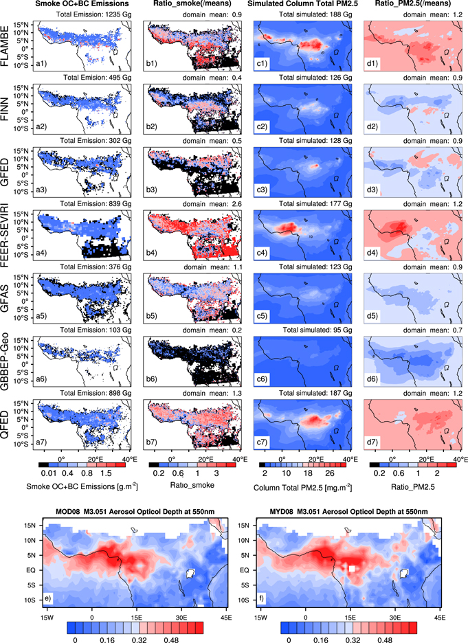
Figure 1. Comparisons among FLAMBE, FINNv1.0, GFEDv3.1, FEER-SEVIRIv1.0, GFASv1.0, GBBEP-Geo and QFEDv2.4 for (a1–a7) monthly total smoke OC + BC emissions (unit: g m−2) during February 2010. The plot is made at the native resolution for corresponding emission inventory; (b1–b7) the ratio of individual smoke emissions to their means among different inventories (Ratio_smoke); (c1–c7) February mean column total PM2.5 (unit: mg m−2) simulated by WRF-Chem3.5; (d1–d7) the ratio of PM2.5 from different emission inventories to their means (Ratio_PM2.5). (e and f) total column aerosol optical depth (AOD) at 550 nm wavelength from MODIS on Terra and Aqua satellites, respectively, as plotted within the NASA Giovanni interactive visualization system (http://disc.sci.gsfc.nasa.gov/giovanni).
Download figure:
Standard image High-resolution imageA total of seven smoke inventories are used independently to specify the BC and OC emissions: (1) FLAMBE (Fire Locating and Modeling of Burning Emissions inventory; Reid et al 2009), (2) FINNv1.0 (Fire Inventory from NCAR version 1.0; Wiedinmyer et al 2011), (3) GFEDv3.1 (Global Fire Emissions Database version 3.1; van der Werf et al 2010), (4) FEER-SEVIRIv1.0 (Fire Energetics and Emissions Research version 1.0 using fire radiative power (FRP) measurements from the geostationary Meteosat Spinning Enhanced Visible and Infrared Imager (SEVIRI); Roberts and Wooster 2008, Ichoku and Ellison 2013), (5) GFASv1.0 (Global Fire Assimilation System version 1.0; Kaiser et al 2012), (6) GBBEP-Geo (NESDIS Global Biomass Burning Emissions Product; Zhang et al 2012), and (7) QFEDv2.4 (Quick Fire Emissions Dataset version 2.4; Darmenov and da Silva 2013). The key specifics of these emission algorithms are listed in table 1. For those inventories (GFED, FINNv1.0, GFAS, and QFED) that do not present the diurnal cycle of smoke emissions, we applied the diurnal profile based upon the three hourly and daily temporal variability in fire emissions derived from Geostationary Operational Environmental Satellite (GOES) and MODIS (Mu et al 2011). Finally, the emission rates are kept as constant for each hour in every three-hourly interval. FINNv1.0, GFEDv3.1, GFASv1.0, and QFEDv2.4 provide smoke emissions for different constituents (such as OC, BC, PM2.5). For other inventories that do not specifically contain BC and OC emissions (such as FLAMBE, FEER-SEVIRIv1.0, and GBBEP-Geo), this study used the set of emission factors described by Andrea and Merlet (2001) to convert total dry matter burned to BC and OC in GBBEP-Geo, and to obtain the OC and BC emission ratios both relative to PM2.5 and to TPM (total particulate matter, table 1). By multiplying those emission ratios with the corresponding products from the emission inventories, OC and BC emissions for FLAMBE and FEER-SEVIRIv1.0 are obtained as well.
Table 1. Intercomparisons of different smoke emission inventories used in this study.
| Category | Method | Data | Resolution | Fire data source | References | Fields |
|---|---|---|---|---|---|---|
| Bottom-up approaches | Fuel consumption and burned area based | FLAMBE | 1 ∼ 5 km, hourly | MODIS/GOES | Reid et al (2009) | PM2.5 |
| FINNv1.0 | ∼1 km2, daily | MODIS | Wiedinmyer et al (2011) | BC,OC, PM2.5,etc | ||
| GFEDv3.1 | 0.5° × 0.5° Monthly | TRMM-VIRS/ATRS; MODIS | van der Werf et al (2010) | BC,OC, PM2.5, etc | ||
| FRP-based with land cover specific conversion factors and emission factors | GFASv1.0 | 0.5° × 0.5°, daily | MODIS | Kaiser et al (2012) | BC,OC, PM2.5, etc | |
| GBBEP-Geo | 3 ∼ 4 km, hourly | GOES (SEVIRI in Africa) | Zhang et al (2012) | Total dry mass | ||
| Top-down approaches | FRP-based with satellite AOD constraint | FEER-SEVIRIv1.0 | 1° × 1°, hourly | MODIS/SEVIRI | Ichoku and Ellison (2013) | Total particulate matter |
| QFEDv2.4 | 0.25° × 0.3125°, or 0.1° × 0.1° daily | MODIS | Darmenov and da Silva (2013) | BC, OC, PM2.5, etc |
Eight sets of simulations are performed for each month, with the first not considering any fire emissions and the rest respectively incorporating seven different emission inventories (as mentioned above). In the model, the injection height of smoke (only OC + BC) emissions is specified as 650 m above the surface (Yang et al 2013). The 1°× 1° National Center for Environmental Prediction (NCEP) 6 h Final Analysis (FNL) data are used for initializing and specifying the temporally evolving lateral boundary conditions. For all simulations, we provide a spin-up time of one week, and only data during February and November 2010 are analyzed.
3. Results and analyses for February
3.1. From emission source to atmospheric loading
Figure 1 shows the monthly-total smoke OC + BC emissions (g m−2; a1–a7) and monthly-mean simulated column total PM2.5 (mg m−2; c1–c7) during February 2010, along with their ratios to the means among different inventories for smoke emission (b1–b7) and for PM2.5 (d1–d7), respectively. Clearly, all inventories showed the zonal distribution of fire emissions around 0–15°N, along with some in the Congo tropical forest (about 7°S, 15°E) (figures 1(a1)–(a7)). These emissions originate primarily from the predominant human-induced fires related to agricultural, savanna, and deforestation burning in the study region (e.g., Hao and Liu (1994), Johnson et al 2008, Dami et al 2012). Confined within the 0–15°N belt are the three high smoke emission centers situated around 15°W −5°W, 0–10°E, and 15°E–30°E, which also correspondingly render three locations of high concentrations of simulated total PM2.5 (figure 1). Hereafter, these regions are named west, middle and east regions, respectively.
Only FEER-SEVIRIv1.0 produced the strongest emissions in the middle region and far weaker emissions in the east region where the strongest emissions are commonly found for the other emission inventories. As shown in table 1, only FEER-SEVIRIv1.0 and QFEDv2.4 are based on top-down approaches that use satellite measurements of both FRP and smoke AOD. However, the FEER-SEVIRIv1.0 emissions over NSSA region are based on geostationary satellite-sensor (SEVIRI) FRP data in conjunction with FEERv1.0 smoke emission coefficients derived from MODIS FRP and near-source smoke AOD (Ichoku and Ellison 2013). Therefore, the difference between the emission inventories also in part supports the fact that the large uncertainty existing among different satellite retrievals may include the spatial and temporal variation of fires. Furthermore, a qualitative comparison of the model total column OC + BC simulations with total column AOD retrievals from MODIS on Terra and Aqua in February 2010 (figures 1(e) and (f)) show that aerosol concentrations are prominent both in the middle and east regions, with the middle region showing a slightly higher loading; indicating that the various emission inventories spatially reflect relative strengths and weaknesses in capturing emission source strengths by using different approaches.
Considering all the estimates as a whole, the overall mean and standard deviation among different smoke emission inventories are 607 ± 397 Gg, with coefficients of variation (CV defined as ratio of standard deviation and the mean of all inventories) of 65%–68% (table 2). Perhaps due to the adoption of MODIS AOD to constrain their smoke emissions, FEER-SEVIRIv1.0 and QFEDv2.4 have similar total emissions and both are a factor of 2–3 larger than GFASv1.0. The smallest emission estimated by GBBEP-Geo is likely due to its use of a constant conversion factor (0.368 ± 0.015 kg (dry mass) M J−1) (Zhang et al 2012), which is four times smaller than that (1.37 kg (dry mass) M J−1) used in GFASv0 (Kaiser et al 2009). Compared with GBBEP-Geo, the GFASv1.0 algorithm continues to adopt the larger land cover-specific conversion factors, leading to larger smoke emissions (Kaiser et al 2012). Furthermore, the absence of constraining GBBEP-Geo with either MODIS AOD or something similar may be another key reason for its lower emissions. As a result, GBBEP-Geo yields a factor of 8–16 smaller emissions than those indicated by FEER-SEVIRIv1.0 and QFEDv2.4. The MODIS burn-scar mapping method used by GFEDv3.1 cannot detect small fires that burn less than half of its 500 m × 500 m nominal pixel size (Giglio et al 2009). Thus, the larger emission in GFASv1.0 as compared to GFEDv3.1 is mainly due to a higher detection threshold used by the MODIS burned area observation product than those in the underlying MODIS FRP observations (Kaiser et al 2012).
Table 2.
Comparisons among domain-total smoke (OC + BC) emissions (Gg), simulated monthly-mean PM2.5 loadings (Gg), simulated monthly-mean domain-mean AOD, simulated monthly-mean domain-mean smoke effects
| Variables | Smoke (OC + BC) emissions (Gg) | Simulated PM2.5 loadings (Gg) | AOD | ΔSWTOAclr (W m−2) | ΔSWSFCclr (W m−2) | ΔT2(K) | ΔT700(K) |
|---|---|---|---|---|---|---|---|
| FLAMBE | 1235 | 188 | 0.034 | −0.42 (−2.34) | −2.47 (−25.1) | −0.033 (−0.26) | 0.017 (0.096) |
| FINN | 495 | 126 | 0.021 | −0.43 (−1.74) | −1.16 (−12.6) | −0.022 (−0.16) | 0.009 (0.058) |
| GFED | 302 | 128 | 0.022 | −0.38 (−1.43) | −1.32 (−12.3) | −0.030 (−0.20) | 0.010 (0.078) |
| FEER-SEVIRI | 839 | 177 | 0.032 | −0.40 (−2.43) | −2.22 (−15.6) | −0.039 (−0.33) | 0.020 (0.118) |
| GFAS | 376 | 123 | 0.021 | −0.37 (−1.37) | −1.26 (−5.4) | −0.025 (−0.15) | 0.009 (0.062) |
| GBBEP-Geo | 103 | 95 | 0.015 | −0.37 (−1.37) | −0.69 (−2.4) | −0.017 (−0.16) | 0.003 (0.076) |
| QFED | 898 | 187 | 0.034 | −0.35 (−1.74) | −2.48 (−13.4) | −0.048 (−0.28) | 0.020 (0.105) |
Mean
|
607 ± 397 | 146
|
0.026
|
−0.39 ± 0.03 | −1.66 ± 0.72 | −0.03 ± 0.01 | 0.013
|
| Range |
12 | 2 | 2.3 | 1 | 3.6 | 3 | 7 |
| CV |
65% | 25% | 31% | 8% | 43% | 33% | 46% |
Note:
aAll domain-mean smoke effects shown here are only based on those grids with 95% confidence by paired samples t test.
b
 : standard deviation;
cRange: max/min;
dCV(coefficient of variation):
: standard deviation;
cRange: max/min;
dCV(coefficient of variation):  .
.
More spatial discrepancies can be seen in figure 1, in which the ratios of smoke emissions of OC + BC to the means among different inventories (labeled as Ratio_smoke) are shown. North-South gradients of fire emissions differ among different smoke inventories, perhaps driven by the different gradients in vegetation density, fuel type and land cover adopted in these inventories. FLAMBE usually has the largest emissions in tropical Africa with Ratio_smoke > 5. Smaller smoke emissions from FLAMBE and FINN are found in the northern parts of the NSSA than in their southern parts, while the reverse is true for GFED. GFAS and QFED show similar spatial patterns may due to the similar application of MODIS FPR observations in both (Kaiser et al 2012, Darmenov and da Silva 2013). Overall, the domain means of Ratio_smoke averaged only over the grids having fire emissions are 0.9, 0.4, 0.5, 2.6, 1.1, 0.2, and 1.3 for FLAMBE, FINN, GFED, FEER-SEVIRI, GFAS, GBBEP-Geo, and QFED, respectively. The overall mean and standard deviation of Ratio_smoke are 1.00 ± 0.81, with a CV of 81%.
Although FLAMBE, one of the bottom-up approaches, produces larger domain total emissions (1235 Gg) than even the top-down approaches, it does not have the largest domain mean of Ratio_smoke (0.9). This is because of a few very big emissions in FLAMBE. The maximum grid-cell emission of 9.09 g m−2 for FLAMBE as compared to <3.55 g m−2 for the other inventories outweighs its overall smaller emissions, more than FEER-SEVIRI and QFED for instance. Among the different inventories based on their daily total emissions per grid cell (figure 2(a)), FLAMBE cumulative smoke (OC + BC) emission is generally in the middle, and smaller than FEER-SEVIRI and QFED for small to medium values. It is only after including big emissions (>148 mg m−2, i.e., log(OC + BC emission) >5) that FLAMBE becomes larger than those of the top-down approaches. This may be due to a static estimate of 62.5 ha area burned per MODIS hot spot adopted by FLAMBE. Reid et al (2009) shows how this estimate results in over-estimation of fire-affected areas in grassland and savanna landscapes, and under-estimation in densely forested landscapes.

Figure 2. (a) Cumulative smoke (OC + BC) emissions (unit: kg m−2) based on the daily total amounts per grid; (b) daily total smoke OC + BC emissions (unit: Gg); (c) daily mean total PM2.5 simulated by WRF-Chem3.5 over the whole fine domain of interest (unit: Gg), along with the fitting lines and the slope ranges. Comparisons are among FLAMBE, FINNv1.0, GFEDv3.1, FEER-SEVIRIv1.0, GFASv1.0, GBBEP-Geo and QFEDv2.4.
Download figure:
Standard image High-resolution imageFor the monthly-mean column loading of PM2.5 simulated by WRF-Chem3.5, their domain means are 188, 126, 128, 177, 123, 95, and 187 Gg for FLAMBE, FINNv1.0, GFEDv3.1, FEER-SEVIRIv1.0, GFASv1.0, GBBEP-Geo and QFEDv2.4, respectively (figure 1). The overall mean and standard deviation are 146 ± 37 Gg with a CV of 25% (table 2). The PM2.5 loadings are within a factor of 2.4 (taking the smallest one from GBBEP-Geo as base), compared with a factor of 12 difference in the emissions. Moreover, as shown in figure 1, the domain means of Ratio_PM2.5 (i.e., the ratios of simulated PM2.5 loadings to the means among different inventories) are 1.2, 0.9, 0.9, 1.2, 0.9, 0.7, and 1.2 for FLAMBE, FINN, GFED, FEER-SEVIRI, GFAS, GBBEP-Geo, and QFED, respectively. The CV of Ratio_PM2.5 is 20%, much smaller than that of Ratio_smoke (81%). Hence, in terms of quantities over the study domain, the large differences in smoke (OC + BC) emissions are not reflected in the simulated loading of PM2.5.
The results may in part reflect the nonlinearity in the source-receptor relationship. In this relationship, the atmosphere, through diffusion as well as wet and dry deposition processes, generally dampens the effect of differences in the source strength on the atmospheric loadings. This can be more clearly shown in figure 2(c). February is the beginning of the transition time from the dry to the wet season in the NSSA region. Thus, the smoke emissions in February, though much smaller than those in January, obviously decrease with time (figure 2(b)). Correspondingly, the simulated PM2.5 loadings decrease with time as well (figure 2(c)), although there exist some peaks caused by big smoke emission events, e.g., on the 6th–7th February. The slopes of PM2.5 decrease from −3.67 to − 4.77 to −1.39 to − 2.18 and then to −0.30 as the smoke emissions decrease from FLAMBE, FEER-SEVIRI and QFED to FINN, GFED, and GFAS and then to GBBEP-Geo. Clearly those inventories producing larger smoke emissions and thus larger PM2.5 loadings generally have larger damping decrements, inferring the nonlinearity in the source-receptor relationship. In other words, the differences in the total amount of emissions among various emission inventories is mainly due to the large differences in the estimate of emissions from areas of large fire concentrations (figure 2(a)). However, these seemingly large fires are probably constituted by multiples of relatively smaller fires that are very local and only persist for a few days at most. As a result, in regional and monthly averages, the effect of differences in the smoke emissions on the atmospheric loadings is largely dampened, resulting in the CVs of the domain means of PM2.5 loadings and Ratio_PM2.5 within a factor of 2–3. However, at the local scale where the large concentrations of the fires occur, quite different spatial patterns are still found (figure 1). For example, taking the GBBEP-Geo as base, the PM2.5 loading differences can reach up to a factor of 16–33 in the smoke source region with the Ratio_PM2.5 of GBBEP-Geo larger than 0.2.
The surface PM2.5 mass concentration shows a similar contrast with respect to emission as the PM2.5 column loading, and overall, it shows a CV of 37% in the domain and monthly averages (figure S4). In terms of Ratio_SFC_PM2.5 (i.e., the ratios of simulated surface PM2.5 concentration to the means among different inventories), the CV is 23%. However, again, at the local scale, a factor of up to 10–60 difference can be found in surface PM2.5 concentrations.
3.2. Smoke clear-sky radiative impacts
Figure 3 shows monthly-mean modeled aerosol optical depth (AOD) at 550 nm, aerosol absorption optical depth (AAOD, blue contour) at 550 nm overlaid with the map of surface albedo, and the smoke radiative effects on modeled clear-sky net downwelling shortwave (SW) top of atmosphere (TOA) radiative fluxes (ΔSWTOAclr, W m−2) in February 2010. Note that only statistically significant ΔSWTOAclr values (paired samples t test with p < 5%) are shown in figure 3.
The AODs (figures 3(a1)−(a7)) present similar patterns as their corresponding PM2.5 loadings (figures 1(c1)−(c7)). The larger the PM2.5 loadings are, the bigger the AODs. The domain averages of AOD at 550 nm are 0.034, 0.021, 0.022, 0.032, 0.021, 0.015, and 0.034 for FLAMBE, FINN, GFED, FEER-SEVIRI, GFAS, GBBEP-Geo and QFED, respectively. Their overall mean and standard deviation are 0.026 ± 0.008, with a spread of 31%. The relative difference of 2.3 is close to that of the simulated total PM2.5 loadings (2.0), reflecting the first-order linear relationship between aerosol mass loading and its optical depth as well.
Negative ΔSWTOAclr are commonly found with the domain means of –0.42, –0.43, –0.38, –0.40, –0.37, –0.37, and –0.35 W m−2 for FLAMBE, FINN, GFED, FEER-SEVIRI, GFAS, GBBEP-Geo, and QFED, respectively (figures 3(c1)−(c7)). Their mean and standard deviation are –0.39 ± 0.03 W m−2 with a spread of 8%. This can be understood that smoke particles with low or moderate AOD values over the low surface albedo conditions (such as over the ocean and tropical forest region with albedo less than 0.15) (figures 3(b1)−(b7)) generally scatter more solar radiation back-to-space than the parts being absorbed (Wang and Christopher 2006). However, over the bright surfaces, the smoke absorption can be enhanced by strong and multiple reflection of solar radiation between the surface and smoke layer (Ge et al 2014). Hence, over the arid Saharan region (northward of 15°N with surface albedo > 0.3), positive ΔSWTOAclr values are found. Also in smoke source regions with moderate surface albedo (0.2−0.25), AOD is larger and single scattering albedo is low, yielding larger AAOD and absorption and hence large positive ΔSWTOAclr. The cancellation between the smoke negative and positive TOA forcings mentioned above produced only a factor of 1.2 differences in domain-means of ΔSWTOAclr, which is far less than that in smoke emissions.
3.3. Smoke all-sky radiative impacts
At regional scales, the surface temperature change is mainly due to the change of net downwelling SW radiative flux. We show in figure 4 the modeled net downwelling SW radiative fluxes at the SFC both under clear sky (ΔSWSFCclr, figures 4(a1)–(a7)) and all sky (ΔSWSFC, figures 4(b1)–(b7)) conditions. To study the changes of CREs induced by smoke particles, we also show in figures 4(c1)–(c7) the modeled SW CREs at SFC (ΔSWCREsfc, W m−2). The SWCREsfc is defined as  , where
  is the net (downward minus upward) flux,
  designates clear skies, and
 denotes a mixture of clear and cloudy skies. Note that only statistically significant results (paired samples t with p < 5%) are shown in figure 4, which is similar to that of Ge et al (2014).
ΔSWSFCclr generally is more significant than its counterpart at the TOA, because both absorption and scattering of smoke particles result in the extinction of radiation at the surface. Their values can be up to −25.1, −12.6, −12.3, −15.6, −5.4, −2.4 and −13.4 W m−2 for FLAMBE, FINN, GFED, FEER-SEVIRI, GFAS, GBBEP-Geo, and QFED, respectively (figures 4(a1)–(a7)). The locations of large reductions of SWSFCclr coincide quite well with the regions of strong smoke emissions (figures 1(a1)–(a7)), and hence also those of large AODs (figures 3(a1)–(a7)). Overall, the domain averages of ΔSWSFCclr are −2.47, −1.16, −1.32, −2.22, −1.26, −0.69 and −2.48 W m−2 for FLAMBE, FINN, GFED, FEER-SEVIRI, GFAS, GBBEP-Geo and QFED, respectively. Together, their uncertainty range is within a factor of 4, and their mean and standard deviation are −1.66 ± 0.72, with a CV of 43%. This uncertainty range is slightly larger than that of AOD (i.e., 2), possibly reflecting the role of multiple scattering and surface inhomogeneity in the domain averages. Moreover, quite different spatial patterns are still found, especially over the source regions. Taking ΔSWSFCclr for example, their differences based on the different emissions compared to GBBEP-Geo can reach up to a factor of 4–19.
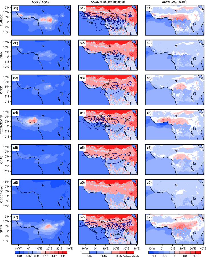
Figure 3. Distribution of monthly averaged quantities in February 2010. (a1)–(a7) Column total modeled aerosol optical depth (AOD) at 550 nm; (b1)–(b7) column total modeled aerosol absorption optical depth (AAOD) at 550 nm (blue contours) over the surface albedo (shaded); (c1)–(c7) modeled net downward SW radiative fluxes at TOA under clear sky ΔSWTOAclr (W m−2). The ΔSWTOAclr shown here are significant at the 95% confidence by paired samples t test. Here  , where, i = FLAMBE/FINN/GFED/ FEER-SEVIRI/GFAS/GBBEP-Geo/QFED.
Download figure:
Standard image High-resolution imageDuring February 2010, there are two distinct synoptic regimes in the domain of interest: one, the dry region north of ∼10°N without clouds at all except at its eastern edge; and the other, the wet region south of ∼10°N with heavy clouds, especially in the ITCZ domain (not shown). As shown in figures 4(b1)–(b7), spatial distributions of ΔSWSFC over the dry region appear to be very similar to those of ΔSWSFCclr due to the lack of clouds. In the wet region, changes in the instantaneous fields of clouds induced by smoke particles can be quite large, although most of them did not satisfy the paired samples t test at the monthly scale (figure not shown). This is mainly due to the high sensitivity of cloud fields to changes in atmospheric circulation, vertical profiles of meteorological fields, vertical stability, and other factors. Nevertheless, over the strong smoke emission regions, significant proportions of ΔSWCREsfc were consistently found to be positive (figures 4(c1)–(c7)), further modifying SWSFC. Positive ΔSWCREsfc increase SWSFC, showing a weakened smoke radiative effect.
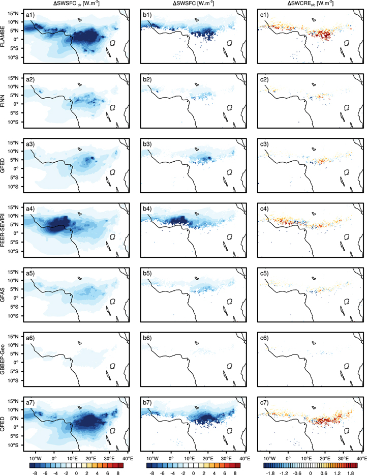
Figure 4. The distribution of monthly averaged quantities in February 2010. (a1)–(a7) difference of modeled net downward SW radiative fluxes at the ground surface under clear sky conditions (ΔSWSFCclr, W m−2); (b1)–(b7) difference of modeled net downward SW radiative fluxes at the ground surface under all sky (ΔSWSFC, W m−2); (c1)–(c7) difference of modeled cloud radiative effects at the ground surface (ΔSWCREsfc,W m−2). Here  , where, F denotes SWSFCclr or SWSFC or SWCREsfc; i the same as figure 3. All the differences shown here are significant at the 95% confidence by t test for paired samples (of Fi
and Fnon_smoke).
, where, F denotes SWSFCclr or SWSFC or SWCREsfc; i the same as figure 3. All the differences shown here are significant at the 95% confidence by t test for paired samples (of Fi
and Fnon_smoke).
Download figure:
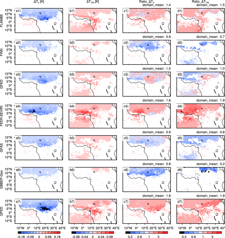
Standard image High-resolution imageFinally, we examine the smoke radiative effects on temperature at 2 m (ΔT2, K, figures 5(a1)–(a7)) and air temperature in the lower troposphere 700 hPa (ΔT700, K, figures 5(b1)–(b7)). Note that only statistically significant differences (paired samples t test with p < 5%) are shown here. Generally speaking, due to the smoke particles' radiative effects, in the smoke emission areas, surface temperature (T2) decreases while temperature in the lower troposphere (e.g., 700 hPa) increases. The strong reductions of T2 are generally caused by the strong decreases in SWSFC, whereas the increases of T700 result from the BC strong absorptions. In addition, the large changes of T700 are generally southeast of those in T2, coinciding with the direction of northeast trade winds. In brief, the decreases of ΔT2 can be up to 0.26, 0.16, 0.20, 0.33, 0.15, 0.16, and 0.28 K, and ΔT700 also show maximal increases with values of 0.096, 0.058, 0.078, 0.118, 0.062, 0.076, and 0.105 K, for FLAMBE, FINN, GFED, FEER-SEVIRI, GFAS, GBBEP-Geo and QFED, respectively. This thermal vertical structure is favorable to a stable atmosphere, and hence reduces the formation of cloud, partially explaining the generally positive changes of SWCREsfc in FLAMBE and QFED (figure 4). The relative small smoke effects on T2 over the ocean are due to the ocean's large heat capacity and latent heat release, and the slight warming may be partly due to the mixing of smoke-absorption-induced warm air in the lower part of the troposphere with the air near the surface (Wang and Christopher 2006).
Figure 5. The distribution of monthly averaged differences in February 2010 for: (a1)–(a7) modeled temperature at 2 m (ΔT2, K); (b1)–(b7) modeled temperature at 700 hPa (ΔT700, K); (c1–c7) the ratio of ΔT2 from different inventories to their means (Ratio_ΔT2); (d1)–(d7) the ratio of ΔT700 from different inventories to their means (Ratio_ΔT700). Here  , where, F is T2 or T700; i the same as figure 3. All the differences shown here are significant at the 95% confidence by paired samples t test, which are also the base for the calculation of domain means.
Download figure:
Standard image High-resolution image
Overall, the mean and standard deviation of ΔT2 and ΔT700 are −0.03 ± 0.01 and 0.013 ± 0.006 K, with a CV of 35% and 51%, respectively. However, we note that the absolute changes in temperature are likely affected by the model configuration in terms of OC and BC ratio, model boundary condition, parameterization schemes for cloud and boundary layers, and relative position between smoke and cloud layers (Feingold et al 2005, Wilcox 2012). While the values of these changes appear small in terms of domain averages, it should be considered that the domain is about eight times larger than the smoke source region (primarily contained within the 4°N–10°N belt). At local scales, the absolute changes of T2 and T700 associated with individual experiments are much larger than their counterparts in domain averages. Among all experiments, a factor of 3 and 7 differences in ΔT2 and ΔT700 are also found, both of which are less than that of smoke emissions (12). Moreover, as shown in figures 5(c1)–(c7) and (d1)–(d7), the domain means of Ratio_ΔT2 (i.e., the ratios of simulated ΔT2 to the means among different inventories) are 1.4, 0.9, 1.0, 1.6, 0.9, 0.8, and 1.6 for FLAMBE, FINN, GFED, FEER-SEVIRI, GFAS, GBBEP-Geo, and QFED, respectively, and those of Ratio_ΔT700 (i.e., the ratios of simulated ΔT700 to the means among different inventories) are 1.5, 0.7, 1.0, 1.9, 0.8, 0.2, and 1.9. The overall mean and standard deviation are 1.17 ± 0.35 with a CV of 30% for Ratio_ΔT2, and 1.14 ± 0.65 with a CV of 56% for Ratio_ΔT700. Those CV are larger than that of Ratio_PM2.5 (<25%), probably due to the fact that only statistically significant values are considered, although they are all significantly smaller than the CV of Ratio_smoke (81%). All the numerical comparisons presented in this study are summarized in tables 2 and 3.
Table 3. Comparisons among domain-means of Ratio_Smoke, Ratio_PM2.5, Ratio_ΔT2, and Ratio_ΔT700. All ratios are compared with the mean values across all emission inventories. The period covered is February 2010.
| Ratio_Smoke | Ratio_PM2.5 | Ratio_ ΔT2 |
Ratio_ ΔT700 |
|
|---|---|---|---|---|
| FLAMBE | 0.9 | 1.2 | 1.4 | 1.5 |
| FINN | 0.4 | 0.9 | 0.9 | 0.7 |
| GFED | 0.5 | 0.9 | 1.0 | 1.0 |
| FEER-SEVIRI | 2.6 | 1.2 | 1.6 | 1.9 |
| GFAS | 1.1 | 0.9 | 0.9 | 0.8 |
| GBBEP-Geo | 0.2 | 0.7 | 0.8 | 0.2 |
| QFED | 1.3 | 1.2 | 1.6 | 1.9 |
Mean
|
1.00 ± 0.81 | 1.00 ± 0.20 | 1.17 ± 0.35 | 1.14 ± 0.65 |
| Range | 13.0 | 1.7 | 2.0 | 9.5 |
| CV | 81% | 20% | 30% | 56% |
Note: aAll domain-mean smoke effects shown here are only based on those grids with 95% confidence by paired samples t test.
4. Results and analyses for November
Although meteorology (including the precipitation belt associated with ITCZ) and emission location and amount are significantly different between February (figure 1 and table 1) and November (figure S1 and table S1), the results obtained for February apply similarly to November. Thus, the atmospheric diffusion and deposition in the model significantly dampen the large difference in smoke emissions, and large differences persist in simulated smoke-related variables and radiative effects at the local scale (figure S2-S8, and table S1 and S2). The main features that reflect differences between February and November include the following:
- Compared to a factor of 16 difference among the seven emission inventories in the increases of their cumulative domain-total smoke (OC + BC) emissions with time (figure S3), only a factor of 3 or less difference exists in those of their simulated column PM2.5 loadings, surface PM2.5 concentrations, smoke forcing at TOA and surface, and smoke effect on temperature at 2 m (figure S2). Such smaller range of the emission effects on modeled atmospheric parameters reflects the nonlinearity in the source-receptor relationship.
- As the season transitions from wet to dry in November, the smoke emissions and PM2.5 loadings gradually increase from the start to the end of November 2010 (figures S2 (b) and (c)), which is opposite to the gradual decrease in February. However, the simulations with FLAMBE emissions also showed a somewhat unique feature that is inconsistent with simulations based on the other emissions. FLAMBE smoke emissions and hence its PM2.5 loadings are significantly large before November 7th. But then, they sharply decrease afterwards until November 20th before increasing again at the end of the month (figures S2 (b) and (c)).
5. Summary and discussions
In this study, by using WRF-Chem3.5 with a fixed model configuration, the sensitivity of the simulated smoke particle loading and smoke direct radiative effects are analyzed for seven commonly used global smoke emission inventories. It is shown that, for the NSSA region, the inventories of smoke organic and BC emissions have 65% and 68% CV during February and November 2010, respectively. However, the CV of simulated monthly mean total PM2.5 loading and hence the AOD are no more than 37% for monthly averages over the entire domain. The large differences in smoke inventories can be primarily attributed to the discrepancies in the estimates of emissions for regions with high fire concentrations. Since such fires are often local and only persist up to a couple of days, their impacts on atmospheric modeling become smaller as they are averaged over larger areas and longer time periods. Consequently, a factor of up to 12–16 relative difference in total smoke (OC + BC) emissions contrasts appreciably with the domain-averaged differences of their atmospheric impact which represents factors of ∼2, 2–3, ∼1, 4–5, ∼3 and 7–13 for column PM2.5 loading, surface PM2.5, AOD, TOA forcing, surface forcing, surface temperature, and temperature at 700 hPa, respectively. However, at monthly and local scales, especially for areas with concentrated burning, significant differences in smoke loadings and the radiative feedback (e.g., a factor of up to 33 in February 2010) can still be found, reflecting the large differences in the spatial and temporal patterns of fire emissions among the different inventories. Hence, to further reduce the uncertainties in regional modeling of smoke effect on climate and air quality, it is critical to resolve the discrepancies in estimating emissions from highly concentrated burning areas. The case studies reported here only presented and analyzed the fire emission differences and their impact on model simulations. Future studies are needed to combine observations with models and field campaign data (if possible) to investigate and possibly mitigate the causes of the large discrepancies among the different emission inventories.
Acknowledgment
This research was supported by the Science Missions Directorate of the National Aeronautics and Space Administration (NASA) as part of an Interdisciplinary Studies (IDS) conducted through the Radiation Sciences Program managed by Hal B Maring. E J Hyer and J Wang also acknowledge the support from the NASA Air Quality Applied Science program managed by John A Haynes. J W Kaiser's contribution was funded by the European Commission through the MACC-II project, contract number 283576, under the EU Seventh Research Framework Programme. C Wiedinmyer would like to acknowledge support from NCAR and US NSF Grant # 121168. The National Center for Atmospheric Research is sponsored by the National Science Foundation. The authors thank Guido van der Werf for providing their emissions datasets, and gratefully acknowledge the Holland Computing Center of the University of Nebraska—Lincoln and their staff for their helpful efforts with modeling.