

Abstract
It is known that carbon dioxide emissions cause the Earth to warm, but no previous study has focused on examining how long it takes to reach maximum warming following a particular CO2 emission. Using conjoined results of carbon-cycle and physical-climate model intercomparison projects (Taylor et al 2012, Joos et al 2013), we find the median time between an emission and maximum warming is 10.1 years, with a 90% probability range of 6.6–30.7 years. We evaluate uncertainties in timing and amount of warming, partitioning them into three contributing factors: carbon cycle, climate sensitivity and ocean thermal inertia. If uncertainty in any one factor is reduced to zero without reducing uncertainty in the other factors, the majority of overall uncertainty remains. Thus, narrowing uncertainty in century-scale warming depends on narrowing uncertainty in all contributing factors. Our results indicate that benefit from avoided climate damage from avoided CO2 emissions will be manifested within the lifetimes of people who acted to avoid that emission. While such avoidance could be expected to benefit future generations, there is potential for emissions avoidance to provide substantial benefit to current generations.
Export citation and abstract BibTeX RIS

Content from this work may be used under the terms of the Creative Commons Attribution 3.0 licence. Any further distribution of this work must maintain attribution to the author(s) and the title of the work, journal citation and DOI.
1. Introduction
It is a widely held misconception that the main effects of a CO2 emission will not be felt for several decades. For example, in a non-peer reviewed setting, Alan Marshall estimated a 40 year lag between greenhouse emissions and elevated temperature1 . Indeed, a co-author on this paper has previously said that 'it takes several decades for the climate system to fully respond to reductions in emissions'2 . Such misconceptions extend beyond the scientific community and have played roles in policy discussions. For example, former US Energy Secretary Steven Chu has been quoted as saying, 'It may take 100 years to heat up this huge thermal mass so it reaches a uniform temperature ... The damage we have done today will not be seen for at least 50 years'3 . On the other hand, Matthews and Solomon (2013) asserted 'Climate warming tomorrow, this year, this decade, or this century is not predetermined by past CO2 emissions; it is yet to be determined by future emissions'. Our results support their assertion that warming that might occur decades from now would be a consequence of future emissions. However, our findings show that past emissions very much influence rates of warming on the time scale of a year or decade following the emission.
In this study, we focus on the amount and timing of global warming associated with a present-day emission of carbon dioxide to the atmosphere—information that is relevant to the projection of the future amount and present value of climate damage expected to occur from the emissions made today. There has been a long tradition of estimating the amount of climate change that would result from various carbon dioxide emission or concentration scenarios (Leggett et al 1992, Ackerman et al 2009, Moss et al 2010) but there has been relatively little quantitative analysis of how long it takes to feel the consequences of an individual carbon dioxide emission.
Uncertainties in the timing and amount of projected additional global temperature increase resulting from an incremental emission of carbon dioxide (CO2) derive from several factors (Huntingford et al 2009). There are carbon-cycle uncertainties associated with the magnitude and timescales of changes in uptake and release of CO2 by the ocean and biosphere (Falkowski et al 2000). There are uncertainties of climate sensitivity associated with the radiative forcing of the emission and feedbacks of the climate system to that forcing that determine the resulting equilibrium global mean temperature change (Knutti and Hegerl 2008). Finally, there are uncertainties of thermal inertia in the climate system associated with the exchange of heat between the atmosphere and the surface and deep oceans which influences the timing of climate change (Winton et al 2010). Two such recent intercomparison projects together contain estimates of our three uncertainty factors from suites of state-of the-art models.
2. Methods
In this analysis, we combine modeling data from a carbon-cycle modeling project (Joos et al 2013) with data from the Coupled Model Intercomparison Project phase 5 (CMIP5) (Taylor et al 2012) to evaluate the climate response to a pulse input of CO2 and its associated uncertainty. Fits to a collection of CO2 responses to pulse releases, performed by Joos et al (2013), are used here to provide an uncertainty range for our understanding of the carbon cycle. Simple models of global temperature response, tuned using CMIP5 simulations of an abrupt quadrupling of CO2, are used to represent and parse the uncertainty ranges for climate sensitivity and ocean thermal inertia.
2.1. Carbon-cycle response characterization
As a part of a carbon-cycle model intercomparison project (Joos et al 2013; a CO2-impulse response function model intercomparison project, IRF-MIP), carbon-cycle models, including complex earth system models, earth system models of intermediate complexity and simple box models, were used to project future changes in CO2 concentration resulting from a CO2 emission. Responses of the atmospheric carbon dioxide concentration to a pulse release of carbon dioxide are well-approximated using a three exponential fit. To characterize the carbon cycle uncertainty associated with the global temperature response to a carbon dioxide emission today, we use fits to the time series of carbon dioxide concentrations from the IRF-MIP experiment's 15 ensemble members (Joos et al 2013) (see supplementary table S1).
For the simulations analyzed here, a 100 GtC pulse of carbon dioxide was released into a system in equilibrium with an atmosphere with a background concentration of 389 ppm CO2. (Annual average atmospheric CO2 content averaged 389 ppm between 2010 and 2011; when we use 'today' in this work, we are referring to this time (Dlugokencky and Tans n.d).) The size of this release was well suited to characterizing carbon-cycle response in these models, but because the release amount was relatively small, the internal model variability dominated the forced response to the carbon dioxide pulse release in all of the coupled climate models included in the ensemble, resulting in a multi-model mean time series for global mean temperature with several local maxima (Joos et al 2013). Therefore, IRF-MIP was ill suited to characterize with confidence the time to maximum warming following an individual carbon dioxide emission. However, this signal-to-noise issue can be resolved by combining the IRF-MIP data with the CMIP5 results.
2.2. Climate system response characterization
Using standard protocols as part of CMIP5, coupled atmosphere–ocean modeling groups projected future changes in global mean temperature resulting from changes in atmospheric CO2 concentration. While the CMIP5 protocol did not include simulations in which a single pulse of CO2 was emitted into the atmosphere, it did include an abrupt4xCO2 simulation. Modeling groups projected the climate change that would occur in response to a step function change in atmospheric CO2 concentrations (Taylor et al 2012).
To characterize both the uncertainty in climate sensitivity and in the thermal inertia of the climate system, we use fits to the time series of global temperature change from the CMIP5 abrupt4xCO2 experiment's 20 ensemble's members (see supplementary table S2). To characterize the climate sensitivity uncertainty range, we use an approach devised by Gregory et al (2004). At least two studies (Andrews et al 2012, Caldeira and Myhrvold 2013), have applied this approach to the CMIP5 multi-model ensemble, and here we use estimates of equilibrium climate sensitivity from a quadrupling of atmospheric CO2 from Caldeira and Myhrvold (2013). These estimates are numerically similar to those provided by Andrews et al (2012) but are accompanied by consistent functions representing the pace of warming for each model.
Unlike climate sensitivity, the thermal inertia of the ocean cannot be described by a single number, but requires some representation of an underlying physical model. Both two-box (Held et al 2010, Geoffroy et al 2012) and one-dimensional heat-diffusion (Hansen et al 1984, MacMynowski et al 2011) have been widely used to characterize the thermal response of more complex climate models. In this study, we characterize the thermal response uncertainty range using whichever of the two underlying physical models better fits the approach to equilibrium for each atmosphere–ocean model used in the CMIP5 abrupt4xCO2 simulations (Andrews et al 2012). For details see the supplementary information. Relevant parameters for the temperature models tuned to each CMIP5 model are documented in table 1. while we assume in our analysis that the climate sensitivity and ocean thermal inertia are independent, there could be correlations introduced by the process of constraining the model behavior to match historical data, though in our analysis this correlation is very weak (R2 = 0.0537).
Table 1. Best-fit ocean model parameters for CMIP5 models based on two-box and 1D diffusion models. The 'better fit' model was used in our study. The climate sensitivity parameter, effective vertical diffusivity and better fit model were first presented in Caldeira and Myhrvold (2013).
| Two-box model (2-exp) | One-dimensional model (1D) | |||||
|---|---|---|---|---|---|---|
| Model | Climate sensitivity parameter (λ) (W m−2 K−1) | Land/ocean-mixed layer effective heat capacity (C) (108 J m−2 s−1 K−1) | Thermocline/deep-ocean effective heat capacity (C0) (108 J m−2 s−1 K−1) | Effective exchange rate (γ) (W m−2 K−1) | Effective vertical diffusivity (κ) (104 m2 s−1) | Better fit model |
| BCC-CSM1.1 | 1.15 | 1.97 | 19.1 | 0.806 | 0.355 | 2-exp |
| BCC-CSM1.1(m) | 1.23 | 1.94 | 16.2 | 0.785 | 0.295 | 1D |
| CanESM2 | 1.03 | 1.95 | 20.8 | 0.699 | 0.338 | 1D |
| CSIRO-Mk3.6.0 | 0.63 | 1.69 | 22.0 | 0.917 | 0.444 | 2-exp |
| FGOALS-g2 | 0.73 | 2.12 | 27.7 | 0.726 | 0.43 | 1D |
| FGOALS-s2 | 0.90 | 1.90 | 37.6 | 0.781 | 0.59 | 2-exp |
| GFDL-CM3 | 0.76 | 1.93 | 21.4 | 0.854 | 0.417 | 2-exp |
| GFDL-ESM2G | 1.00 | 1.34 | 39.7 | 0.766 | 0.591 | 2-exp |
| GFDL-ESM2M | 1.06 | 1.75 | 40.6 | 0.864 | 0.689 | 2-exp |
| INM-CM4 | 1.47 | 2.42 | 69.9 | 0.714 | 0.713 | 2-exp |
| IPSL-CM5A-LR | 0.78 | 3.16 | 36.6 | 0.554 | 0.464 | 1D |
| IPSL-CM5A-Mr | 0.81 | 2.54 | 26.7 | 0.662 | 0.418 | 2-exp |
| IPSL-CM5B-LR | 1.04 | 1.74 | 20.1 | 0.739 | 0.332 | 1D |
| MIROC5 | 1.55 | 1.98 | 40.5 | 0.872 | 0.692 | 2-exp |
| MIROC-ESM | 0.92 | 2.59 | 36.7 | 0.731 | 0.571 | 2-exp |
| MPI-ESM-LR | 1.12 | 1.87 | 22.2 | 0.790 | 0.395 | 2-exp |
| MPI-ESM-Mr | 1.18 | 1.92 | 21.9 | 0.768 | 0.382 | 2-exp |
| MPI-ESM-P | 1.24 | 1.75 | 21.7 | 0.816 | 0.391 | 2-exp |
| MRI-CGCM3 | 1.26 | 2.38 | 19.4 | 0.761 | 0.362 | 1D |
| NorESM1-M | 1.10 | 2.13 | 33.4 | 1.035 | 0.747 | 2-exp |
2.3. Coupled carbon-climate approximation
A combined approximation of the climate system's response to a present-day CO2 pulse emission can be obtained by using a standard convolution integral approach similar to that of Shine et al (2005), convoluting the carbon cycle and climate system responses:

where RΔT is the global temperature response to a step-change in atmospheric CO2, as defined by one of the two models described above and in the supplementary methods;  is the 3-exponential atmospheric carbon dioxide response to a present-day pulse release. This yields 15 estimates of the carbon cycle response to a unit emission, 20 estimates of climate sensitivity, and 20 simplified models of the thermal inertia of the climate system, giving us 6000 possible combinations of these three factors. We limit our analysis to the first century of warming in order to remain within the scope of any simulation in either ensemble.
While the response of the carbon cycle to pulse releases of CO2 may vary with the size of the emission pulse as they grow far beyond 100 GtC (Eby et al 2009), we here assume a linear scaling factor, α, to account for the difference in the magnitude of the forcing response for the pulse release simulated as opposed to the step change in CO2 concentration (i.e., 100 GtC from 389 ppm versus abrupt4xCO2). We assume that the global temperature response of the climate system is linear enough that RΔT as derived from the abrupt4xCO2 simulations is representative of the response to more complex forcing perturbations. This assumption is supported by contemporary analyses (Andrews et al 2012, Good et al 2013). Our results are relevant to CO2 releases of less than 100 GtC where these linear approximations are most likely to be valid.
The range of model results in model intercomparison projects is often taken as indicative of scientific uncertainty in scenario-based projections (Tebaldi and Knutti 2007). When we say 'very likely' (Mastrandrea et al 2010) in presenting our results, our statements related directly to the distribution of model results. It is possible that all models are biased in a similar fashion and thus the probability that real values will lie outside of our stated uncertainty ranges may be underestimated. In addition, the approach does not account for the fact that models with highest rates of ocean carbon uptake are likely to also have high rates of heat uptake—these properties of the Earth system are independent according to our method. Nevertheless, because these models represent the scientific community's best effort to quantitatively represent known physics and biogeochemistry, these model results are at least indicative of current scientific uncertainty.
3. Results and discussion
Across the 6000 combined projections, there is a high degree of concordance on the overall magnitude and general shape of global warming resulting from a CO2 emission (figure 1). A pulse emission of CO2 results in a stepwise increase in atmospheric CO2 content, followed by a slow decrease as the CO2 is taken up by the oceans and terrestrial biosphere. Global temperature rises in response to the CO2 forcing, but with a lag of about a decade due to the thermal inertia of the upper layers of the ocean. The maximum temperature is reached when the ever-decreasing rate of warming in response to the increase in radiative forcing is balanced by the slowly decreasing magnitude of radiative forcing of atmospheric CO2.
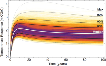
Figure 1. Temperature increase from an individual emission of carbon dioxide (CO2). Time series of the marginal warming in mK (=milliKelvin = 0.001 K) per GtC (=1015 g carbon) as projected by 6000 convolution-function simulations for the first 100 years after the emission. Maximum warming occurs a median of 10.1 years after the CO2 emission event and has a median value of 2.2 mK GtC−1. The colors represent the relative density of simulations in a given region of the plot.
Download figure:
Standard image High-resolution imageFigure 2 shows, for all 6000 projections, the distributions of the amount of time after the emission that it takes to reach the maximum temperature anomaly caused by a CO2 emission (ΔTmax), the magnitude of ΔTmax, and ΔT as a fraction ΔTmax at 100 years after the emission. The median estimate of the time until maximum warming occurs is 10.1 years after the CO2 emission, with a very likely (90% probability) range of 6.6–30.7 years (figure 2(a)). We find a median estimate of the maximum amount of warming caused by a CO2 emission during the first century after the emission (ΔTmax) is 2.2 mK GtC−1, with a very likely range of between 1.6 and 2.9 mK GtC−1 (figure 2(b); supplementary table S3). This range is in keeping with contemporary estimates of transient climate response to cumulative carbon emission obtained in a number of studies (Collins et al 2013), though our metric is time-dependent so the values are not directly comparable.

Figure 2. Frequency distributions of time to ΔTmax, magnitude of ΔTmax, and ΔT at year 100 relative to ΔTmax. The frequency distribution functions, based on all 6000 simulations, for: (a) the time until the maximum temperature increase achieved in the first 100 years after a CO2 emission (ΔTmax) is reached (in years), (b) the magnitude of ΔTmax (in milliKelvins per gigatonne carbon), and (c) the fraction of that warming remaining 100 years after the emission. Vertical axis units are the multiplicative inverse of the horizontal axis units.
Download figure:
Standard image High-resolution imageConsistent with a long list of previous work (e.g., Archer 2005, Matthews and Caldeira 2008, Solomon et al 2009), figures 1 and 2 show that while the temperature consequences of CO2 emission materialize more quickly than commonly assumed, they are long lasting. The fraction of maximum warming still remaining one century after an emission has a median value of 0.82, with a very likely range of 0.65–0.97 (figure 2(c)). (Note that after one century, temperatures are still increasing in 119 of the 6000 simulated time series (i.e., have not reached ΔTmax) and therefore, if the simulation datasets available and analysis were extended for a longer time period, 2% of simulations would have fractional values greater than one.) In addition, even if the globally averaged maximum effect of an emission may be manifested after one decade, the results may vary spatially. For example, continued polar amplification may result in later a maximum warming effect at high latitudes.
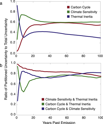
We partition uncertainty in the temperature increase following an emission into three independent factors: uncertainty in the carbon cycle, equilibrium climate sensitivity and thermal inertia (figure 3). As our central case for our sensitivity study, we choose the one convolution simulation out of the 6000 available that minimizes the least-squares difference with the numerically-determined median warming trajectory shown in figure 1. Climate sensitivity is the largest individual contributing factor to temperature response uncertainty, but the combined effect of all three uncertainty sources is a considerably larger range. There has been considerable focus on the 'high tail' on equilibrium climate sensitivity estimates (Roe and Baker 2007), but this analysis suggests that carbon cycle uncertainty contributes nearly as much to the high tail of warming as climate sensitivity does. We find that carbon cycle uncertainty increases steadily relative to other factors over time, and that the ratio of carbon cycle uncertainty to that associated with climate sensitivity and thermal inertia together is about 0.42 after a decade, but 0.72 after a century (figure 3(a)). This suggests that the relative magnitude of carbon cycle uncertainty to uncertainty associated with physical uncertainties is larger than previous similar analyses have found (Huntingford et al 2009).
Figure 3. Partitioned uncertainty over time. The fraction of 90% (very likely) uncertainty range remaining if different contributors to overall uncertainty were reduced to zero: (a) uncertainty of two factors is reduced to zero, with no reduction in uncertainty in the third (labeled) factor, (b) uncertainty of one factor is reduced to zero, with no reduction in uncertainty in the other two factors.
Download figure:
Standard image High-resolution image
Substantially reducing the uncertainty about the effect of an emission will require more than just constraining climate sensitivity. While climate sensitivity is the largest contributor to total uncertainty, even if climate sensitivity uncertainty were reduced to zero, more than 70% of total uncertainty about the magnitude of warming remains 100 years after the emission (figure 3(b)). Removing uncertainty for any one factor will only decrease total uncertainty about the magnitude of warming by 20–30%. This is also true for reducing uncertainty about the timing of warming; even eliminating all uncertainty about thermal inertia—the largest contributor to uncertainty about the time until ΔTmax—only reduces the total uncertainty range about timing by 44%.
Our analysis provides an estimate of the timing and amount of incremental warming that would be caused by CO2 emitted today. These estimates span the uncertainty range of model results, yet are simple enough to be employed in a broad range of climate change assessment applications. In supplementary methods we describe the development of simple 3-exponential fits to the solid lines shown in figure 1, and provide relevant coefficients in table 2. These curve fits could be useful for approximating the temperature increase resulting from CO2 emissions in alternative scenario analyses, economic modeling, or other exercises that require a simplified but physically robust representation climate system's response to CO2 emissions. However, care should be used when applying these representations under conditions far from the current state, because carbon-cycle dynamics and physical climate system response both vary with background atmospheric CO2 concentration. At higher CO2 concentrations, the ocean takes up CO2 more slowly, leaving more CO2 in the atmosphere. However, at higher CO2 concentrations, that additional CO2 also produces less radiative forcing. These two effects are opposite in sign and of approximately the same magnitude, so there is first-order cancellation (Caldeira and Kasting 1992), but detailed results will differ. In addition, these results are only appropriate for the representation of the temperature response in the first century after a CO2 emission. The multi-century scale warming effects have not been extensively explored in fully coupled AOGCMs that include a carbon cycle (Pierrehumbert 2014), but some preliminary work suggests that some warming effects of an emission may extend well beyond the first century (Frölicher et al 2014).
Table 2. Fit coefficients for a three-exponential function representing the marginal temperature response to a present day emissiona.
| a1b | a2b | a3b | τc | τ2c | τ3c | rmsb | ||
|---|---|---|---|---|---|---|---|---|
| Median | −2.308 | 0.743 | −0.191 | 2.241 | 35.750 | 97.180 | 0.005 | |
| Likely | Lo | −2.121 | 0.535 | 0.318 | 2.663 | 14.960 | 78.316 | 0.002 |
| (>66%) | Hi | −0.777 | −1.884 | 0.539 | 0.048 | 2.659 | 41.581 | 0.003 |
| Very likely | Lo | −2.327 | 0.812 | 0.410 | 3.084 | 8.384 | 50.173 | 0.004 |
| (>90%) | Hi | −1.507 | −1.447 | 0.727 | 0.432 | 3.628 | 105.899 | 0.006 |
| Virtually certain | Lo | −2.314 | 1.066 | 0.498 | 3.255 | 8.849 | 112.671 | 0.009 |
| (>99%) | Hi | −2.264 | −1.367 | 6.830 | 0.689 | 7.458 | 1000.000 | 0.016 |
| Minimum | Lo | −2.147 | 1.011 | 0.463 | 3.012 | 8.186 | 101.242 | 0.016 |
| Maximum | Hi | −2.278 | −2.405 | 13.811 | 0.630 | 9.106 | 1000.000 | 0.018 |
aThe functional form is:  bUnits of mK GtC−1.
cUnits of years.
bUnits of mK GtC−1.
cUnits of years.
While the maximum warming effect of a CO2 emission may manifest itself in only one decade, other impact-relevant effects, such as sea level rise, will quite clearly not reach their maximum until after the first century (see, e.g., figure 2(c) of Joos et al (2013)). For many impacts, such as changes to natural ecosystems, degradation is the result of the cumulative effects of consecutive years of warming or precipitation change (Parmesan and Yohe 2003). Ice sheet melting can persist for thousands of years following a warming (Huybrechts et al 2011). As such, even if maximum warming occurs within a decade, maximum impact may not be reached until much later. From this perspective, Steven Chu's statement that today's damage 'will not be seen for at least 50 years' may well be accurate.
4. Conclusions
Our analysis implies warming from an individual carbon dioxide emission can be expected to reach its peak value within about a decade and, for the most part, persist for longer than a century. There is substantial uncertainty in both the amount and timing of this warming, and while the largest contributor to this uncertainty is equilibrium climate sensitivity, there are substantial contributions from the carbon-cycle and climate system thermal inertia. Carbon-cycle uncertainties make a contribution to the 'high tail' of the temperature response distribution that is comparable to climate sensitivity's contribution.
Carbon dioxide emissions are long-lasting and generate multi-century and multi-millennial commitments (Archer et al 2009). On the multi-century scale, some authors have suggested that the climate response to a CO2 emission can be regarded as a nearly immediate step function change followed by relatively constant warming that persists for centuries (Matthews and Caldeira 2008, Solomon et al 2009, Matthews and Solomon 2013). Our results provide additional evidence that on time scales substantially longer than a decade, the warming from a CO2 emission can be approximated by a step function increase in temperature that then remains approximately constant for an extended period of time. Under this framing, the amount of climate change is critical to estimating climate damage stemming from an emission, and delays in warming may be regarded as relatively unimportant. Extreme forms of this perspective even suggest that the timing of emission is unimportant, and cumulative emissions are most relevant to the policy process (Zickfeld et al 2009).
On the other hand, economic evaluations of costs and benefits typically take timing into consideration, discounting gains and losses in the future relative to those of the present day (Nordhaus 1992) and thereby placing much greater significance on the warming experienced in the first decades after an emission. Some have suggested that the benefits of emissions avoidance will be felt nearly immediately (Matthews and Solomon 2013), whereas others have emphasized that benefits of emissions avoidance will accrue primarily to the next generation and beyond (Myhrvold and Caldeira 2012).
The primary time lag limiting efforts to diminish future climate change may be the time scales associated with political consensus (Victor 2011) and with energy system transitions (Smil 2010), and not time lags in the physical climate system. While the relevant time lags imposed by the climate system are substantially shorter than a human lifetime, they are substantially longer than the typical political election cycle, making these delays and their associated uncertainties important, both economically and politically. Nonetheless, our study indicates that people alive today are very likely to benefit from emissions avoided today.
Acknowledgments
The authors thank K Taylor and three anonymous referees for helpful comments that improved this manuscript.
Footnotes
- 1
- 2
- 3