
Abstract
Recent food crises have highlighted the need to better understand the between-year variability of agricultural production. Although increasing future production seems necessary, the globalization of commodity markets suggests that the food system would also benefit from enhanced supplies stability through a reduction in the year-to-year variability. Here, we develop an analytical expression decomposing global crop yield interannual variability into three informative components that quantify how evenly are croplands distributed in the world, the proportion of cultivated areas allocated to regions of above or below average variability and the covariation between yields in distinct world regions. This decomposition is used to identify drivers of interannual yield variations for four major crops (i.e., maize, rice, soybean and wheat) over the period 1961–2012. We show that maize production is fairly spread but marked by one prominent region with high levels of crop yield interannual variability (which encompasses the North American corn belt in the USA, and Canada). In contrast, global rice yields have a small variability because, although spatially concentrated, much of the production is located in regions of below-average variability (i.e., South, Eastern and South Eastern Asia). Because of these contrasted land use allocations, an even cultivated land distribution across regions would reduce global maize yield variance, but increase the variance of global yield rice. Intermediate results are obtained for soybean and wheat for which croplands are mainly located in regions with close-to-average variability. At the scale of large world regions, we find that covariances of regional yields have a negligible contribution to global yield variance. The proposed decomposition could be applied at any spatial and time scales, including the yearly time step. By addressing global crop production stability (or lack thereof) our results contribute to the understanding of a key aspect of global food availability.
Export citation and abstract BibTeX RIS

Content from this work may be used under the terms of the Creative Commons Attribution 3.0 licence. Any further distribution of this work must maintain attribution to the author(s) and the title of the work, journal citation and DOI.
1. Introduction
Adequately feeding the world growing population is the global food system foremost function [1]. Since the beginning of the green revolution, increase rates of agricultural output outpacing global population growth rates have fueled the idea that increasing average production is the answer to global food insecurity. Persistence of endemic hunger however challenges the view that profusion of food is sufficient to ensure worldwide stable access to food [2]. Available global assessments further suggest that undernourishment can affect an additional fraction of the population because of interannual variability of production or during crises (e.g., in 2008). In fact, definitions of global food security have evolved to integrate a stability pillar [3].
The challenge of feeding nine billion people at the 2050 horizon has led many recent studies to focus on long-term trends in productivity [4–6] e.g., by estimating average crop yield increase rates [7, 8]. The emphasis placed on the need to increase productivity trends may however tend to overshadow the importance of also considering accompanying interannual variability. This is despite the latter having been recognized as an important factor influencing price volatility [9, 10]. Accounting for interannual variability of future crop yields in equilibrium models and food balance sheets is likely to increase the reliability of food security studies conclusions [11–13].
Several factors may influence yield interannual variability (hereafter YIV), e.g., climate variability [14–16], farmers' practices [14], or economic incentives [9, 10]. Evidently, the level of temporal variability varies greatly depending on the spatial scales at which it is considered [18]. As a first step, this study describes and analyzes YIV at the subcontinental (geographical world regions) and global scale while leaving aside the issue of the underlying explanatory factors. We focus on three key staple crops and one oil crop i.e., maize, wheat, rice (roughly 92% of total cereal production and 661 million hectares in 2012) and soybean.
Specifically, we address two main questions: how different are world regions in terms of YIV; how does the distribution of cultivated areas among world regions affect global YIV?
To make progress, we define a practical measure of YIV (as the variance of yield residuals) and propose a mathematical decomposition that analytically connects global to regional YIV using three information-rich components (section 2). These are (i) a term proportional to the Simpson diversity index (adapted to measure the relative spatial concentration of production in time), (ii) a term depending on the proportions of cultivated areas allocated to regions of above or below average variability and (iii) a weighted sum of the co-variation between regional yield residuals.
Definitions and the analytical development are presented in section 2 along with the dataset. We apply the decomposition in section 3 and uncover the various underlying trade-offs between components of global YIV. In the discussion (section 4) we expose the contrasts between maize, rice, soybean and wheat yield variability and identify the way global yields would be impacted by changes in land use distribution.
2. Material and methods
2.1. Data
Our dataset includes yield and area time series extracted from the FAOSTAT database [19] for four crops species (maize, rice, soybean and wheat) in all FAOSTAT world regions excluding Melanesia, Micronesia, Polynesia and the Caribbean. We thus consider 17 regions for maize, rice and soybean and 18 for wheat (adding Northern Europe). For most regions the time series extend from 1961 to 2012, except in Central Asia (1992–2012).
We define a yield residual  at year t in a region i as

where  is the observed yield (t/ha) and
  is the expected yield value (t/ha) at year t for a given crop in the ith region. Values of
  are estimated using linear, quadratic or cubic regression models. These models are fitted by ordinary least squares, using the R function lm for each yield time series for each crop species at each geographical unit. The model showing the lowest Akaike Criteria (AIC) is selected to detrend yield time series for each crop and each region. We check for absence of autocorrelation in residuals.
For simplicity, we use the word yield 'anomaly' instead of yield 'residual' to characterize detrended yield time series.
We estimate regional yield interannual variability  for a given crop from the variance of regional yield anomalies as

where  is time-average of anomalies (equal to zero by construction). Note that we also compute a standard deviation for each region
  (figure 1.)
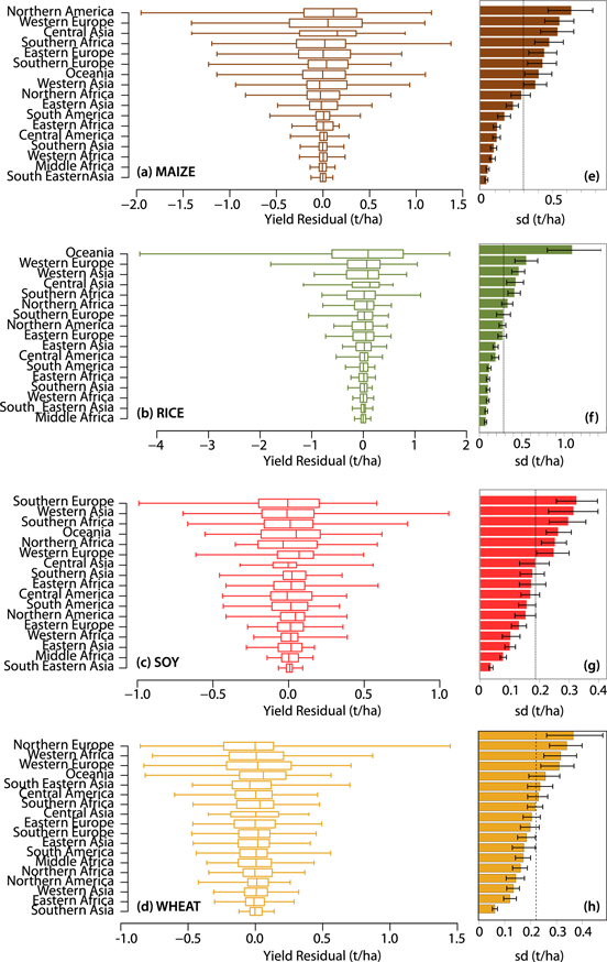
Figure 1. (a)–(h). (a)–(d). Box plot of yield anomalies (t/ha). Yield anomalies calculated each year between 1961 and 2012 in all producing regions for maize (a), rice (b), soybean (c) and wheat (d). Box plot range corresponds to the 25th, 50th and 75th percentile and arms extend to minimum and maximum values. Regions are ordered according to decreasing variance (calculated as time-average squared anomalies). (e)–(h). Barplot of yield anomaly standard deviation (t/ha) (equation (2) for 1961–2012. 95% Confidence intervals are calculated from 1000 bootstrap iterations. Dotted line is the average standard deviation for all regions.
Download figure:
Standard image High-resolution image2.2. Analytical decomposition of global yield anomalies
We define below a mathematical expression (equation (5)) connecting regional yield anomalies (equation (1)) to global yield anomalies. We calculate the variance of global yield in a second step (equation (6)). Two limit cases are presented at the end of the section.
Let Rt be the global anomaly (i.e., the difference between global yield and global expected yield value at the world level at time t) for a given crop,  , with
  ,
,  ,
,  the proportion of the world cultivated area allocated to the ith region at year t, and N the total number of regions where the considered crop is grown.
The squared value of  is defined by:
As
we have

with  (squared regional yield anomaly in t2/ha2),
  , the product of regional yield anomalies in regions i and j, i.e.,
  in t2/ha2.
We introduce  as the difference between squared yield anomaly in the ith region
  and the mean of squared regional yield anomalies over all regions at each time step (i.e., the interregional yield variance
  ), further noted
  (t2/ha2). This difference can be negative (or positive) if the squared residual in a given region is higher (smaller) than the average over all regions.
We then get from equation (3)
As the Simpson diversity index can be defined by  , we finally get from (4)

Equation (5) decomposes squared global yield anomalies at a given year as a sum of three terms (in t2/ha2):  ,
,  , and
, and  . The yield variance at the global scale is then defined by the time average of squared global yield anomalies
  expressed as
Equation (6) relates global yield variance V to three additive components  . Each of these components depends on yield anomalies and on the proportions of cultivated areas and are all expressed in t2/ha2. Note that although none of the individual components actually corresponds to a variance, their sum does. The three components can be estimated independently using regional yield anomalies and proportion of cultivated areas derived from FAOSTAT data. Importantly we also compute values of
  , i = 1,..., N, i.e., the regional contributions to component 2, for each region, but only present area proportions for the most important regions in figure 3.
There are a few limit cases of equation (5) that can be explored. In particular we investigate two extreme situations in terms of land allocation. In the first limit case, all cultivated areas are allocated in one region only (region k):
Limit case 1:
In this case, the global yield variance is simply equal to the yield variance in the region where all the cultivated area is allocated (region k).
In the second limit case, all cultivated areas are evenly distributed among the N world regions:
Limit case 2:
As

we get
In this second limit case, we thus get  and
and  . The value of
  thus depends on the mean of squared regional yield anomalies and on co-variation between yield anomalies in distinct regions. If the covariance between
  and
and  is negligible across time, then
  .
.
Regional yield anomalies and proportions of cultivated areas are calculated from FAOSTAT data for the period 1961–2012. This enables us to calculate regional yield variance  (equation (2)) for each crop, and global yield variance V (equation (6)) with its three components, for each crop over the entire time period (see result section) and over shorter time windows (see SI). Note that a comparison of the results obtained for different time periods shows that the respective values of each components are fairly stable in time.
3. Results
3.1. Levels of yield variability are regionally contrasted
Figure 1 shows the time distribution of regional yield anomalies (equation (1)) for maize, rice, soybean, and wheat (panels a to d). These distributions differ among crop species; differences between minimum to maximum yield anomalies range from 2 (t/ha) for soybean to 6 (t/ha) for rice. Maize and rice regional yield anomaly distributions are asymmetrical towards negative values in the topmost region (i.e., North America and Oceania respectively). Soybean yield anomaly distributions are more similar among regions and wheat asymmetry is linked to one region only with highest yield positive anomaly (i.e., Northern Europe).
Standard deviations of yield anomalies calculated per region per crop over the totality of the time period are also displayed (figures 1(e)–(h)). We find large inter-regional differences especially for rice (yield anomaly standard deviation ranging from 0.073–1.094 t/ha) but also for maize (0.047–0.638 t/ha). Standard deviation confidence intervals (calculated from 1000 bootstrap samples) indicate that regions with highest standard deviation are significantly different from the average standard deviation calculated over all regions (dotted line in figures 1(e)–(h)). Groups of regions that are significantly above average are clearly distinct from the ones that are below average with a third group of regions not being significantly different from average (this is one region for maize, four for rice and soybean and six for wheat). Although some regions do not significantly differ in terms of standard deviation, at least two groups of regions with low and high standard deviations can be identified for each crop.
3.2. Concentration of production higher for soybean and rice than for wheat and maize
Figure 2 illustrates the evolution of cultivated area proportions for regions totalizing at least 75% of global cultivated areas over the study period. The Simpson diversity index which was first developed to characterize species diversity [20] is here used to reflect the evolution of the spatial repartition of cultivated areas among world regions (see inserts in figure 2). The index indicates heterogeneity for high values (i.e., a concentration of production in a few regions) and homogeneity at low values (i.e., a more even distribution of hectares among regions). Highest values of the Simpson index are obtained for soybean and to a lesser extent, rice. It indicates that soybean production is the most spatially concentrated followed by rice with maize and wheat exhibiting comparable levels of heterogeneity in particular at the end the time period. While maize and rice Simpson indices remained somewhat constant during the study period, wheat and most notably soybean Simpson indices show a decreasing trend with some differences. Wheat index shows a monotonous decreasing trend followed by a stabilizing period. On the other hand, the spatial spread of soybean production appears to be marked by three consecutive periods.
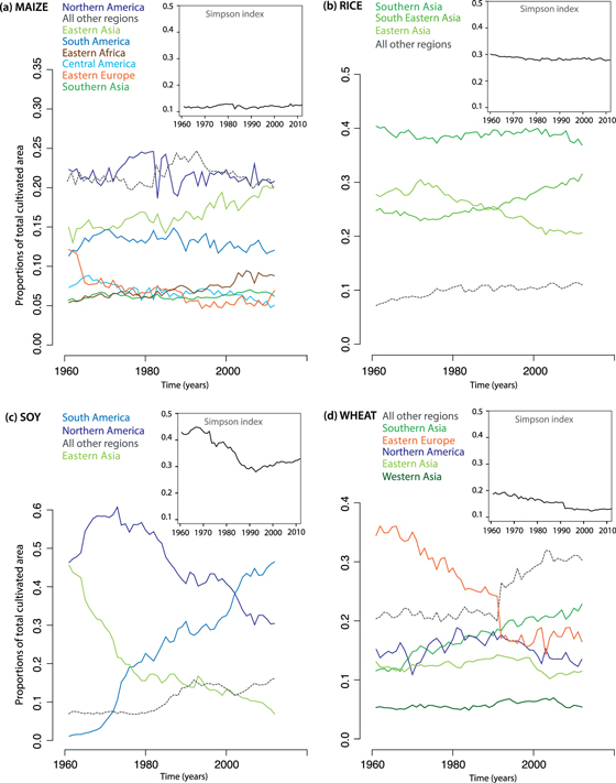
Figure 2. (a)–(d). Spatial repartition of cultivated areas among regions. Time series of area proportions for cultivated land for regions totalizing at least an average of 75% of total cultivated areas during the study period. This is six regions in total for maize (a), 5 for wheat (d) and 3 for rice (b) and soybean (c). Insert: Simpson index time series for each species (1961–2012).
Download figure:
Standard image High-resolution imageThese patterns can be explained by the dynamics of area proportions (figures 2(a)–(d)). A close look at the Simpson index for soybean reveals a short increase until 1968 (reflecting an increase in the concentration of production in North America) followed by an overall decrease of the index during 1968–1993. The trend observed in 1968–1993 is due to the accession of South America to significant proportions of total cultivated areas (i.e., from less than 2% in 1960 to almost 30% in 1993, see figure 2(c)). After 1993, proportions of soybean areas allocated to Eastern Asia and to North America still follow a decreasing trend, and the soybean production becomes more and more concentrated in South America (about 45% of the total soybean area in 2010). But, although the replacement of Eastern Asia and North America by South American areas initiated a concentration of production, soybean production is less concentrated in 2012 than it was in 1961 when only two regions totalized above 90% of total areas (i.e., Eastern Asia and North America for about one fourth of actual surfaces).
American maize production occupies more than 20% of global maize areas over the totality of the time period. Towards the end of the period, Eastern Asia maize areas (China among three other countries) also reach about 20% of world maize areas and, together with Eastern Africa areas (ranging from Ethiopia to Madagascar) replacing South and Central America and Eastern Europe areas (figure 2(a)). The actual repartition of land among regions is fairly spread out with a total of seven regions producing 84% of global maize production on 78% of total areas, on average over the study period. Note that maize Simpson index has the lowest values of all crop species (i.e., values ranging between 0.11 and 0.13), suggesting that maize production is less spatially aggregated than the other crops.
Rice is predominantly produced in Asia; in Eastern Asia (about 40% of total production on average over the study period), Southern Asia (∼29%) and Southeastern Asia (∼23%). Rice production is spatially concentrated as revealed by the relatively high Simpson index (about 0.3 over the time period); on average, the three above-mentioned regions totalized above 90% of the production on above 90% of global cultivated areas (figure 2(b)). The most important region in terms of cultivated areas and production is Southern Asia covering a stable 40% of global areas throughout the period. A notable development is the increase -in particular after the 1990 s- in total and in proportion of South Eastern Asia rice areas (especially Thailand and Indonesia, among 11 countries). Eastern Asia areas remained somewhat constant but decreased in proportion (figure 2(b)).
Five regions totalize about 76% of global wheat areas over the study period. Wheat Simpson index decreases from about 0.2 to about 0.13 over the time period. Wheat production is thus more spread out than rice and soybean and about equivalent to maize. Wheat prominent feature is the collapse of Eastern Europe areas in 1992. Area proportions show an increase followed by a decrease in both North America and Eastern Asia. Southern Asia (India and eight other countries) is the only major producing region with a sharp increase of its cultivated area during the study period, representing about 23% of global surfaces at the end of the time period.
3.3. Key components of global yield variability differ among crops
The order and values of global YIV components differ among crop species (figures 3(a)–(d)). In particular, maize YIV decomposition is very different from that of rice, soybean and wheat. In the following we focus on maize and rice because of their contrasted variance decomposition.
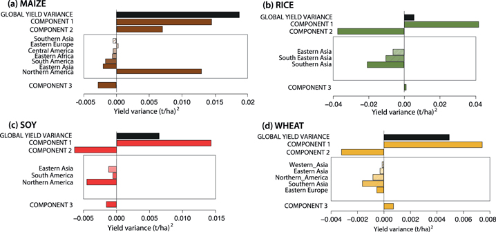
Figure 3. (a)–(d). Decomposition of global yield variability. Time series of global yield anomalies are calculated from equation (1) as the yearly difference between observed global yield value and the weighted sum of regional yield expected values. Using equation (5) we decompose squared values of global anomalies into three components. Component 1 is the product of average squared yield anomalies over all region and the Simpson index applied to area proportions; Component 2 is the weighted sum of the difference between squared anomalies in a single region and the average over all regions and Component 3 is the weighted average of yield anomaly covariance between regions. Time-average values of the three components are plotted here (in t2/ha2). Component 1 is positive by construction but components 2 and 3 can display negative values (if most production is occurring in regions of above average variability and if regional yield anomalies are negatively correlated respectively). Rectangle insert: we show regional values of component 2 for the most important regions (the color density of plotted regions reflects decreasing area proportions). The decomposition is applied to maize (a), rice (b), soybean (c) and wheat (d).
Download figure:
Standard image High-resolution imageComponent 1, (equation (6)), is bigger for rice (0.042) than maize (0.014). This is because of higher Simpson index values for rice compared to maize (i.e., rice is more than twice as spatially concentrated as maize). Also, average squared anomalies over all producing regions,
  is slightly bigger on average for rice than maize (mainly because of the 2008 rice yield anomaly in Oceania).
Component 2 describes how regional yield anomalies compare to the inter-regional average. This component is positive and small for maize and strongly negative for rice (figures 3(a)–(b)). Component 2 is negative (positive) when regions with large proportions of cultivated area show small (high) squared regional yield anomalies. For rice, the three major producing regions are located in Asia and all show a negative regional component  (figure 3(b)) meaning that these three regions have smaller squared anomalies than average. For maize, North America is both the largest and the most variable producing region (figure 1(e)). Consequently, the value of the regional component
  (equation (5)) calculated for North America is positive and much higher that the regional components calculated for the other maize producing regions (figure 3(a)).
Component 3  , equal to the weighted sum of all yield regional covariances, is negative for maize (i.e., on average negative yield anomalies tend to be compensated by positive anomalies in other maize producing regions) and positive and small for rice.
Soybean and wheat yield variance components are similar (figures 3(c), (d)). Global variances V are lower than those of maize and rice. Component 2 is negative for both crops indicating that the majority of the production is located in regions with below-average squared anomalies, in particular North America for soybean (the most important region on average although outpaced by South America post 2000, see figure 2) and Southern Asia for wheat. Soybean regional yield anomalies tend to be negatively correlated thus decreasing global yield variance. Wheat component 3 values are very close to zero. Note that the relative importance of each component within the decomposition is unchanged when varying the time window of the classification (figure S1).
3.4. Effect of a uniform repartition of cultivated areas on global yield variance
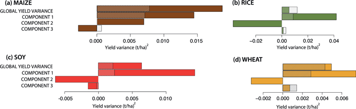
Figure 4 shows values of global variance and of its components in case of a uniform repartition of cultivated areas among regions. These results correspond to the second limit case described in section 2.2. In this case, the same proportion of cultivated area is allocated to each region, Simpson index is equal to its minimum value (i.e., 1/N), and component 2 is equal to zero. This limit case is theoretical as proportions of cultivated area in all regions cannot be equal in reality. Our underlying hypothesis is that a more even distribution of land will decrease global yield variance by distributing risk over a large number of regions. We use this limit case to determine how much global yield variance could be reduced or increased by using an even repartition of cultivated areas at the world scale.
Figure 4. (a)–(d). Limit case: equipartition of cultivated areas among all world regions. Decomposition of global yield variability for a theoretical uniform distribution of cultivated areas among world regions (i.e., Simpson index takes its lowest possible value: 1/N, with N the total number of regions). The theoretical decomposition is presented in hatched whereas the actual decomposition is presented in colored bars for maize (a), rice (b), soybean(c) and wheat (d). Note that a uniform cultivated area distribution automatically sets component 2 to 0 (as developed in limit case 2, see methods section). Global yield variance is decreased for maize, soybean and wheat but increased for rice.
Download figure:
Standard image High-resolution image
Results show that an even distribution of cultivated land decreases maize and soybean global variance to roughly half and a third of its original value respectively. It also decreases, but to a lesser extent, global wheat variance. On the contrary, rice global yield variance is increased in case of a uniform land use distribution (figure 4). These contrasted results are due to the fact that an allocation of 1/Nth of the total areas to all N regions has two effects on the decomposition. First, component 2 is automatically brought to zero (see methods section, limit case 2). Second, component 1 automatically decreases, because the Simpson index is at its lowest value. Component 1 is then proportional to inter-regional yield variance  .
.
Component 2 was initially highly negative for rice, and this negative value is set to zero when using of a uniform distribution of cultivated area. The use of a null value for component 2 instead of a negative one is only partially compensated by a decrease of component 1, and the global yield variance for rice is thus higher compared to its original value (figure 4(b)). For maize, component 2 was originally highly positive, and this positive value is set to zero when using of a uniform distribution of cultivated area. For this crop, the use of a null value for component 2 instead of a positive one leads to a strong decrease of the global maize yield variance (figure 4(a)). Although component 2 was initially negative for soybean and wheat, an even repartition of cultivated lands leads to a smaller global yield variance for these two crops. This is due to the fact that the reduction of component 1 is able to compensate the increase of component 2 for these two crops, resulting in an overall variance decrease (figures 4(c)–(d)).
4. Discussion and conclusion
Our results fill an important gap in the large-scale analysis of yields by identifying, for the time, key drivers of global yield anomalies. We show that a global yield anomaly can be expressed as a sum of three components describing spatial spread of global production, allocation of cultivated areas in regions of strong versus weak variability, and covariance of local yield anomalies in distinct regions. Our decomposition exposes several trade-offs underlying global crop yield variability. We show for instance that a high degree of concentration of rice-cultivated lands can be offset by lower than average regional yield variability. On the contrary, for maize, the allocation of a high proportion of cropland to a region with above-than-average variability leads to high yield variability at the world level. Covariance of regional yield anomalies can compensate (e.g., as displayed by component 3 for maize) or add up (e.g., component 3 positive value in soybean decomposition) to increase or decrease global yield variance.
We show that much of the global variance in maize yield anomalies can be attributed to North America. North America alone totalizes between 35 and 45% of the world maize production on 21% of the total maize surfaces on average. North America is also the region with highest maize yields with expected values around ten tons per hectare in 2012, i.e., north America is the single most important maize-producing region since 1961. But North America is also the region with highest standard deviation of maize yield anomalies. Several factors may be involved. Three climatic events particularly standout in North America yield anomaly time series: 1983, 1988 and 2012 i.e., three major corn belt drought [21] associated with roughly 27, 32 and 25% yield loss respectively. These events explain approximately one-fourth North American residual standard deviation. High instability of yields in this region explains why maize is the only crop species showing a positive value for component 2. This result has an important consequence; because of the high and positive value of component 2 in North America, a—theoretical—even allocation of surfaces would roughly half global yield variance of maize.
Rice production on the other hand is in a situation of low risks. The three largest rice-producing regions are Eastern, Southeastern and Southern Asia, and all three regions are characterized by relatively low yield standard deviations. The decomposition of global rice yield anomalies shows that the positive value of component 1 is almost fully canceled by the strongly negative value of component 2. This reflects the fact that rice is production is highly aggregated spatially (leading to a high value of component 1) but, produced in regions where yields anomalies are lower than average (leading to a strongly negative value of component 2). This result explains why a theoretical even distribution of land among world regions would actually increase rice global yield variance (figure 4). Note though, that if one of the three main rice-producing regions were to increase in variance, the decomposition would suggest that the overall variability could sharply increase because of the strong concentration of rice production.
South America, North America and Eastern Asia are the three main soybean-producing regions since 1961, with a significant decrease of cultivated areas in the latter over the study period. North and South America show very similar levels of regional yield variability (for all risk measures, see table S1). In comparison, yield standard deviation is slightly lower in Eastern Asia. In all three regions, yield standard deviations are close to average (figure 2) and, for this reason, value of component 2 is small.
The results obtained for wheat are to close to those obtained for soybean; main producing regions show smaller squared anomalies than average, leading to negative value of component 2. Among the major producing regions, Southern Asia shows the smallest yield standard deviation (the same ranking is obtained with other risk measures, see SI). If wheat area proportion continues increasing in Southern Asia for example at the level of Eastern Europe at the beginning of the time period, this could contribute decreasing global yield variance providing that it is not compensated by increased spatial concentration of production.
The proposed decomposition is valid at any time scale, for long or short period of time or at the yearly time step. In our calculations we average the components over 1961–2012 (equation (6)). In this study we operate at the scale of large FAO world regions. Although the expression of our decomposition is valid at any spatial scale (e.g., countries), the relative weights of the three components are likely to change depending on the considered scale, with smaller scale decomposition assuredly heightening the contribution of regional yield correlations [10, 18].
Our study also reveals that all FAO regions have contrasted yield standard deviation. Standard deviation is a popular measure of yield instability [22], but other risk metrics can be used as well, such as percentiles or expected shortfall [23]. The robustness of our regional ranking to the chosen risk metric is analyzed in the supplementary materials (table S1(a)–(d)). Note that our results (i.e., the classification of regions according risk levels) are consistent for all risk measures.
A series of factors can be invoked to explain differences in regional yield variability. Fluctuating environment are know to impact crop yield year-to-year variability, in particular regional climate [14–17, 22, 24–26]. Crop management [17] and agronomic practices such as irrigation [25], changes in varieties [25, 27, 28], increased use of inputs can also affect the range of interannual yield variations. It may be hypothesized that abiotic or biotic stress on crop growth can be offset by the large range of responses available to farmers in economically developed regions. No clear evidence of lower variance in such regions is found here. Also, there is little evidence that highest variance are significantly determined by higher yield levels. A significant relation can be found for maize and rice to a lesser extent. Average yields explain a significant portion of total deviance in maize but a very small fraction of the between region differences for rice, soybean and wheat (figure S2). No significant relation is found between yield standard deviation and average area proportions. Key studies have focused on characterizing the temporal variation of yield variability (see for example [29–31]). Our decomposition can be used to understand the dynamics of crop yield variability but the evolution in time of regional yield variance is beyond the scope of this study.
This paper focuses on the effect of the distribution of cultivated area on yield variability, but land use obviously also has an effect on global yield and production average. From a production standpoint it may seem optimal to allocate areas to the most productive regions. Some of our results suggest a possible antagonism between yield variability and average production, at least for some crop species (e.g., maize). Analyzing tradeoffs between production levels, land use and yield stability is of interest to policy makers because it helps defining land use scenarios offering interesting compromises between high production and low risk. In the future, our decomposition could be applied at various scales to identify situations where global crop yield variance could be reduced by using a more even geographical distribution of cultivated areas.
Acknowledgments
The authors would like to thank two anonymous reviewers for providing helpful comments on an earlier version of this manuscript and Lucien Bourgeois, Aude Barbottin, Marie-hélène Jeuffroy and Jean-Marc Meynard for useful discussions.