
Abstract
Recent studies have suggested that measurements of the diurnal temperature range (DTR) over Europe may provide evidence of a long-hypothesized link between the cosmic ray (CR) flux and cloud cover. Such propositions are interesting, as previous investigations of CR–cloud links are limited by data issues including long-term reliability and view-angle artifacts in satellite-based cloud measurements. Consequently, the DTR presents a further independent opportunity for assessment. Claims have been made that during infrequent high-magnitude increases (ground level enhancements, GLE) and decreases (Forbush decreases, Fd) in the CR flux significant anti-correlated DTR changes may be observed, and the magnitude of the DTR deviations increases with the size of the CR disturbance. If confirmed this may have important consequences for the estimation of natural climate forcing. We analyze these claims, and conclude that no statistically significant fluctuations in DTR (p < 0.05) are observed. Using detailed Monte Carlo significance testing we show that past claims to the contrary result from a methodological error in estimating significance connected to the effects of sub-sampling.
Export citation and abstract BibTeX RIS

Content from this work may be used under the terms of the Creative Commons Attribution 3.0 licence. Any further distribution of this work must maintain attribution to the author(s) and the title of the work, journal citation and DOI.
1. Introduction
It has been proposed by Dragić et al (2011, 2013) that a long-debated link between solar activity and terrestrial cloud properties may be reliably detected by applying composite analysis techniques to observations of the diurnal temperature range (DTR—a quantity defined as the difference between observed daily minimum and maximum surface air temperatures). Dai et al (1999) have shown that the DTR can be used as a proxy for cloud cover, and so detections of significant DTR changes corresponding to solar variability (e.g. during changes in the CR flux) could provide compelling support for a hypothesized CR–cloud link (Dickinson 1975, Pudovkin and Veretenenko 1995, Svensmark and Friis-Christensen 1997). Two theoretical microphysical mechanisms have been proposed which may account for a link between CR-induced atmospheric ionization and changes in cloud properties (Stozhkov 2003), these are the so-called direct effect of atmospheric ionization on aerosol nucleation and growth (Ney 1959, Dickinson 1975, Carslaw et al 2002), and an indirect effect of atmospheric ionization on cloud properties via the global electric circuit (Khain et al 2004, Tinsley et al 2000, Harrison and Ambaum 2008, Nicoll and Harrison 2010). Of these mechanisms the direct effect is better understood, with modeling and laboratory experiments indicating that atmospheric ionization changes experienced over a solar cycle are insufficient to induce significant global changes in aerosol and cloud properties (Pierce and Adams 2009, Kirkby et al 2011, Snow-Kropla et al 2011, Kazil et al 2012, Dunne et al 2012). It is less clear how the indirect effect may influence cloud cover, as cloud variations resulting from indirect ionization effects may be spatio-temporally inhomogeneous (Tinsley 2008), and thus even the net sign of cloud change resulting from variations in atmospheric ionization is uncertain.
It is possible that a CR–cloud link may be more apparent in DTR data than from direct satellite-retrieved cloud observations, as the satellite cloud data were not intended for long-term monitoring and are subject to numerous issues affecting data reliability (Stubenrauch et al 2013a, 2013b). Specifically, these issues include biases from top-down viewing angles (Minnis 1989, Loeb and Davies 1996, Campbell 2004), artificial deviations due to changes in calibration satellites (Norris 2005, Evan et al 2007, Várnai and Marshak 2007), spurious trends connected with instrumental degradation and changes in the number of observing satellites (Evan et al 2007), biases related to changes in viewing time (Salby and Callaghan 1997), and issues in regions of overlapping cloud (Tian and Curry 1989, Rozendaal et al 1995). Such limitations may complicate or even prevent the detection of any potential low-amplitude solar signals (Laken et al 2012b). Indeed, a range of ground-based studies have demonstrated evidence of a significant low-amplitude CR–cloud link (Harrison and Stephenson 2006, Harrison et al 2011), whereas detailed analysis of satellite-retrieved cloud data has consistently yielded negative (or false-positive) results (Laken et al 2012b, Krissansen-Totten and Davies 2013).
As an additional advantage, DTR data are available over a longer time period than satellite cloud data (for which observations approximately began in 1983). Consequently, by using DTR data we may examine relatively more infrequent high-magnitude variations in the CR flux in order to improve the potential signal-to-noise ratio of our analysis. If a solar–cloud link were validated, it would have important implications regarding natural climate forcings, implying that over the past century the contributions of natural forcings may have been underestimated while anthropogenic forcings may have simultaneously been overestimated. Such arguments remain central to persistent controversial claims regarding the magnitude of natural climate change which has occurred over the past century (e.g. Svensmark 2007, Rao 2011, van Geel and Ziegler 2013, van Kooten 2013).
Composite analysis (also known by the names of Chree, superposed epoch analysis, and conditional sampling) refers to the technique of isolating small amplitude signals from relatively larger background variability by the successive accumulation of data (Chree 1913, 1914, Forbush et al 1983, Singh et al 2006, Laken and Čalogović 2013). In this work, we focus on variations in the composite mean calculated from single events obtained during infrequent, daily timescale, high-magnitude variations in the CR flux, a parameter which has been continuously observed by neutron monitors (NM) around the world for the past sixty years (Simpson 2000). The composite methods and Monte Carlo (MC) analysis approaches employed throughout this work are described in detail in Laken and Čalogović (2013).
Dragić et al (2011) reported that significant reductions in the DTR have been observed over Europe following the most intense Forbush decrease (Fd) events, these are sudden daily timescale reductions in the background CR flux (Forbush 1937, Cane 2000). Furthermore, recent work by Dragić et al (2013) suggest that the inverse conditions, ground level enhancement (GLE) events (a high-magnitude increase in the CR flux (Meyer et al 1956)), produce increases in the DTR. Interestingly, the authors showed that the absolute magnitude of the DTR changes increases with the magnitude of both the Fd and GLE events analyzed, and they considered that together these results make for convincing evidence of a solar signal present in the DTR data.
These results are scrutinized in this paper using detailed Monte Carlo (MC) significance testing methods to identify the probability (p) of achieving the DTR variations observed during Fd and GLE events. In particular, we highlight how to accurately evaluate the statistical significance of the composite samples following the sub-sampling of Fd and GLE events, which adds a further level of complexity to the MC analyses performed.
2. Data and methods
2.1. Meteorological station data
The DTR is calculated as the daily minimum surface temperature (Tmin) subtracted from the daily maximum surface temperature (Tmax). The surface level temperature data were obtained from the daily summaries of meteorological stations in the Global Historical Climate Network (GHCN) maintained by the National Oceanic and Atmospheric Administration (NOAA) National Climatic Data Center (NCDC) available at www.ncdc.noaa.gov/cdo-web/datasets. DTR was calculated for each calendar date of each meteorological station individually over a time period from 01/01/1950 to 31/12/2011 where data is available, with units in degrees Celsius (° C).
For consistency, we have used the same 189 European region meteorological stations as listed in the on-line supplementary material of Dragić et al (2011). An example of the daily values of DTR from Dnipropetrovśk station (Ukraine), is shown in figure 1(a). In this figure all DTR values are plotted by their day-of-year (DOY) on the x-axis, with a cubic spline fit to the data points (red line) smoothed with a seven-day binning. Additionally, the ±1 standard error (SE) range around the mean is over-plotted (blue shaded region). This demonstrates the seasonal profile of Dnipropetrovśk station and it is essentially equivalent to figure 2 presented in Dragić et al (2011). Seasonal profiles for all 189 stations utilized in this work are available online. The shape of these profiles depends on local climatic factors (Dai et al 1999) and consequently large differences can be seen over the seasonal profiles of individual stations. The case shown in figure 1(a) represents the profile of a typical temperate continental climate. By averaging the 189 stations together data from numerous climatic regimes has been combined.
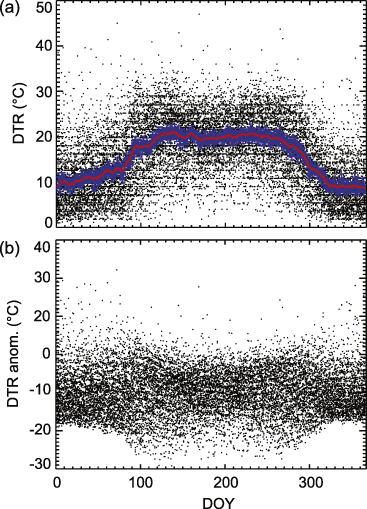
Figure 1. Example of DTR data (in ° C) from a single meteorological station (Dnipropetrovśk, ID 345040, 48.6° N, 35.0° E, 143 m asl) during 1950–2010 with values plotted by their day-of-year (DOY) occurrence. Panel (a) shows the daily DTR values (points), along with an over-plotted blue shaded region to indicate the ±1 standard error range around the mean. A cubic spline (CS) fit to the data is also shown (red line) smoothed with a seven-day binning. In panel (b) the CS fit has been subtracted from the individual data points to construct an anomaly.
Download figure:
Standard image High-resolution image2.2. Filtering methods and noise reduction prior to composite generation
Our hypothesis test is as follows: the null hypothesis (H0) is that CR changes do not have a detectable impact on the mean DTR values over Europe, while our alternate hypothesis (H1) is that CR changes do have a detectable impact on the mean DTR values over Europe. In order to maximize the chance of detecting a CR–cloud link we must construct our experiments to both isolate a clear signal (where we define signal as DTR variations statistically connected to CR changes) and to minimize the noise (where we define noise as DTR changes unrelated to a signal).
If we were to leave variations at timescales greater than those connected with our hypothesis test we may reduce the sensitivity of our experiment. Seasonal variations are clearly unrelated to a signal, and thus all similar investigations of a CR–DTR link so far have removed seasonal DTR variations prior to constructing composites (Dragić et al 2011, 2013, Laken et al 2012a, Erlykin and Wolfendale 2013). Dragić et al (2011, 2013) achieved their seasonal de-trending by subtracting cubic spline (CS) fits from the mean DTR data for each DOY and each meteorological station separately, as shown in figure 1(b) (resulting values referred to here as anomalies). However, we find that this method of anomaly creation is problematic in this instance due to the broad distribution of data points over the years of accumulated data (see figure 1(a)). Large differences between the DOY values, particularly during the periods of seasonal transition (i.e. as summer becomes winter and vice versa) results in a non-uniform distribution of anomalies (figure 1(b)). Consequently, generating anomalies for each station in this manner and averaging them across all meteorological stations to produce a time series of European region DTR values, creates data with an unequal variance through time, and may result in the production of composites strongly influenced by noise.
We have attempted to improve upon this approach of anomaly creation by subtracting a 21-day moving average (high-pass filter, HPF) from the daily DTR value of each meteorological station, and then these resulting values (also referred to here as anomalies) are averaged to generate a European region DTR time series, this method was used in Laken et al (2012a) and Erlykin and Wolfendale (2013). The benefits and limitations of applying a 21-day moving average filtering method are discussed in detail in Laken and Čalogović (2013). Essentially, this method enables DTR changes at timescales concerned with the hypothesis testing to persist while reducing or completely removing variations at timescales unrelated to our hypothesis test. For a hypothesized tropospheric response to the Fd and GLE events the upper-limit time response is estimated to be ≤7 days (Arnold 2006). By identifying a theoretical upper-limit response time to ionization changes we are able to apply a corresponding HPF, thereby potentially increasing the experimental signal-to-noise ratio and increasing the likelihood that a signal may be detected. However, due to the filtering applied, our experiment is unable to reliably draw conclusions regarding DTR variations at timescales >7 days as variations at timescales above 1/3rd the width of the filter become increasingly attenuated; they are completely removed at timescales greater than the width of the HPF. A further limitation of the HPF method is the addition of overshoot artifacts, this issue is discussed in Laken and Čalogović (2013).
The number of meteorological stations contributing to the mean European region DTR value occasionally shows strong decreases, which we find coincide with notable changes in the distribution of DTR anomalies. This is shown in figure 2, which presents the daily number of contributing stations (a value between 0 and 189) over the available data period (figure 2(a)), plotted below this is the corresponding DTR anomaly calculated from the HPF method (figure 2(b)). Several periods of large DTR variations can be seen, occurring in conjunction with reductions in the contributing stations. Consequently, to remove these spurious variations from the analysis we have excluded data for which there were ≤50 stations contributing to the daily mean. These are highlighted in red in figure 2(b), and altogether occur on a total of 383 days (1.7% of the data).
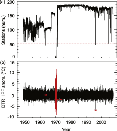
Figure 2. Panel (a) shows the number of meteorological stations for which surface temperature measurements are available from the 189 stations used in Dragić et al (2011) over the available data period. In (b) the weighted mean DTR anomaly calculated by subtracting a 21-day moving average (HPF) from the observed record is shown. Data points for which there are ≤50 station measurements available are highlighted in red; these points are excluded from the following analysis.
Download figure:
Standard image High-resolution imageThe distributions of DTR anomalies obtained from the removal of cubic spline (CS) fits and 21-day high-pass filters (HPF) are presented in figure 3. These distributions are obtained from 100 000 Monte Carlo (MC) simulations comprised of composites of n = 20 random dates using two separate DTR anomaly time series, one generated by the removal of a CS fit (figure 3(a)) and another by the removal of a HPF (figure 3(b)). In both cases the composite means were weighted by the standard error (SE) calculated from the distribution of DTR anomalies on each day from individual stations. Median values of the CS and HPF anomaly distributions are −0.08 ° C and −0.05 ° C respectively, and full-width-at-half-maximum (FWHM) values are 0.73 ° C and 0.57 ° C respectively. For further details regarding these MC methods see Laken and Čalogović (2013). From figure 3 it is evident that by using the HPF method we obtain anomalies with a far narrower distribution of values compared to a CS method. The reason for this is twofold: firstly, subtracting the HPF from the data does not create time periods of irregular and high dispersion, such as those created at seasonal transition periods by the CS method. Secondly, variations at timescales unconnected to the hypothesis testing have been removed more effectively than was possible with a CS method. Although the CS method accounts for seasonality, variations which cannot be removed by linear de-trending methods may still exist in the data at timescales longer than those which directly concern the hypothesis testing. The presence of these intermediate timescale fluctuations alters the amount of autocorrelation within a composite and may impact the accuracy of significance testing (Forbush et al 1982, 1983, Singh et al 2006, Laken and Čalogović 2013). Therefore, a relatively higher experimental sensitivity may be achieved by using the HPF-generated anomalies compared to the CS-generated anomalies, as it has reduced noise (more regular dispersion), and reduced autocorrelation (due to an absence of intermediate and long timescale variations).

Figure 3. Histograms of DTR anomalies generated by: (a) the removal of a CS fit, and (b) the removal of a HPF. Values are calculated from the means of 100 000 MC-generated composites of n = 20, weighted by their standard error (SE) values. These data have not been normalized against a base period.
Download figure:
Standard image High-resolution imageThe amount of autocorrelation (persistence) in a dataset may be quantitatively assessed by the Hurst (H) exponent (Hurst 1951, Hurst et al 1965). By using the method of Blok (2000) we estimate the H exponent of the CS and HPF time series anomalies to be 0.82 and 0.30 respectively. This suggests that the CS anomaly time series possesses persistent positive correlation whereas the HPF anomaly shows weak anti-correlation. In this case, the weak anti-correlation results from the generation of data with a static mean: strongly positive values are inevitably followed by strongly negative values and vice versa, as a result the mean values tend towards zero over time. This quantitative assessment of the anomalies provides further confirmation that narrowing of the DTR distribution in figure 3(b) is achieved by the reduction of autocorrelation within the data.
2.3. Creation of composites
For each of the GHCN meteorological stations we have calculated a daily value of DTR by subtracting the recorded surface temperatures Tmin from Tmax. From these data we calculated a simple daily mean of DTR for available stations over the European region, and a daily standard error (SE) from the standard deviation of the station means divided by the square root of the number stations available on each day. The resulting European region daily mean time series was then filtered with a HPF (21-day running average) described in section 2.2 to create an anomaly time series. Each composite constructed in this work is a two-dimensional matrix of this HPF anomaly data, see Laken and Čalogović (2013) for further details regarding the structure of composites. The composite data presented in this work are means of the n dimension at each t-point with the SE calculated using the standard deviation (σ) of the weighted means. The composite means were weighted by the SE associated with the anomaly time series using the method outlined in Bevington and Robinson (1969, p 76).
2.4. Neutron monitor data and selection of Fd/GLE events
The Fd events were identified using the Mt. Washington neutron monitor (NM) data, with a geomagnetic cutoff rigidity Rc = 1.24 GV (44.3° N, 299.7° E), accessible from www.ngdc.noaa.gov/stp/solar/cosmic.html. The GLE events were selected using data from Oulu NM (Kananen et al 1991), with a Rc = 0.81 GV (65.05° N, 25.47° E), obtained from http://cosmicrays.oulu.fi. From these resources we identify the dates and absolute NM deviations of 34 Fd onset events with an intensity of >7% from 1951 to 1995 and 12 GLE events from 1964 to 2012 with an intensity of >10% that did not coincide with another major Fd or GLE event during a ±7-day period and were coincident within the period of our useful DTR data.
We have used the same sampling criteria as described in Dragić et al (2011, 2013) to identify Fd/GLE events for composites, this was done in order to produce comparable results in order to investigate if a significant solar link has indeed been identified. The specific dates are listed in table A.1. In section 3 we present the results of composites constructed from samples of these dates.
It is important to emphasize that GLE events frequently occur in association with Fd events, consequently, of the 22 GLE events with intensities of >10% noted by Kananen et al (1991) since 1966, ten were unsuitable due to the close occurrence of Fd events (<±7 days). Isolation of GLEs from Fd events is important as the ionization effects of these events are inverse. Consequently, improper isolation may result in the compositing of events with weak or negligible atmospheric ionization, lowering the potential signal-to-noise ratio of our experiments.
Numerous investigations have already been made regarding the influence of GLEs on the atmosphere which are relevant to this work. For example, Usoskin et al (2011) calculated the atmospheric ionization associated with specific GLE events in the lower and middle troposphere, and demonstrated that the ionization changes during many GLE events was negligible or even negative at low- and mid-latitude regions due to accompanying Fd events. They also pointed out that the intensity of NM variations during GLE events is not directly comparable to the intensity of atmospheric ionization across the globe: the strongest GLE events (occurring without closely associated Fds) can produce widely varying atmospheric ionization effects, as shown in table 1 of Usoskin et al (2011). By comparing our GLE events (table A.1) to those of Usoskin et al (2011) we find that only 4 of the 12 events are associated with increases in atmospheric ionization of >10% at 10 km in the polar atmosphere. This suggests that even by identifying and compositing the strongest GLE events as detected by ground-based NMs, the atmospheric ionization changes associated with the events may be too small to theoretically result in detectable cloud changes, and therefore may not provide a useful basis to test a hypothesized CR–cloud link. However, despite this we proceed with an analysis of GLE events comparable to that of Dragić et al (2013) in order to comment on their results and investigate their claims.
We note that even if we were to select GLE events with a consideration of calculations of cosmic ray-induced atmospheric ionization from available models (e.g. Desorgher et al 2005, Usoskin and Kovaltsov 2006, Usoskin et al 2010) the analysis would be limited to only several rare events with large atmospheric ionization increases. Investigations of such events have been made, examining possible associations between atmospheric ionization and aerosol development over the polar stratosphere during individual GLEs (Mironova et al 2012, Mironova and Usoskin 2013). As these investigations focused on single events the statistical strength of the results were limited and the widespread applicability of the findings were unclear.
In general, the intensity of atmospheric ionization resulting from Fd/GLE events shows strong spatial variability, approximately increasing with altitude and geomagnetic latitude (Bazilevskaya et al 2008, Čalogović et al 2010). Therefore, strictly in relation to the atmospheric ionization changes induced by Fd/GLE events the surface level European region is not the most optimal location to test for potential CR–cloud linkages, although this limitation is balanced by the relatively high density, frequency, and time span of measurements over the European region (and at surface level) compared to higher latitudes (and higher altitudes).
2.5. Estimating significance from Monte Carlo generated distributions
Our hypothesis is concerned with testing if composites based on Fd and GLE events have a statistically unusual property (in this instance a weighted mean), with respect to random DTR composites of equal size n. We may effectively assess this by using a Monte Carlo (MC) approach. By randomly generating composites of equal size n and repeating this many times it is possible to build up probability density functions (PDFs) of mean values and evaluate the Fd/GLE composite means against these distributions to obtain an exact probability (p) value. Similar approaches have long been used to examine the impacts of solar activity on atmospheric properties (e.g. Schuurmans and Oort 1969). Modern MC-approaches to determine the statistical significance of composites are described in detail in Laken and Čalogović (2013) and references therein. In the following sections we use MC-generated PDFs comprised of 10 000 random composite means to determine the obtained p-values for each individual time step (t) in our Fd/GLE samples. From these PDFs we identify the two-tailed confidence intervals at the p0.05 and p0.01 intervals using a percentile function (i.e. by considering the 0.005/0.995, and 0.025/0.975 percentiles of the PDFs at each t-point). This requires the assumption that it is possible to sample randomly from a DTR anomaly time series to create composites and PDFs for the evaluation of statistical significance, however this is sometimes inadequate as will be discussed in section 3.2.
3. Analysis
3.1. Fd and GLE composites evaluated using MC methods
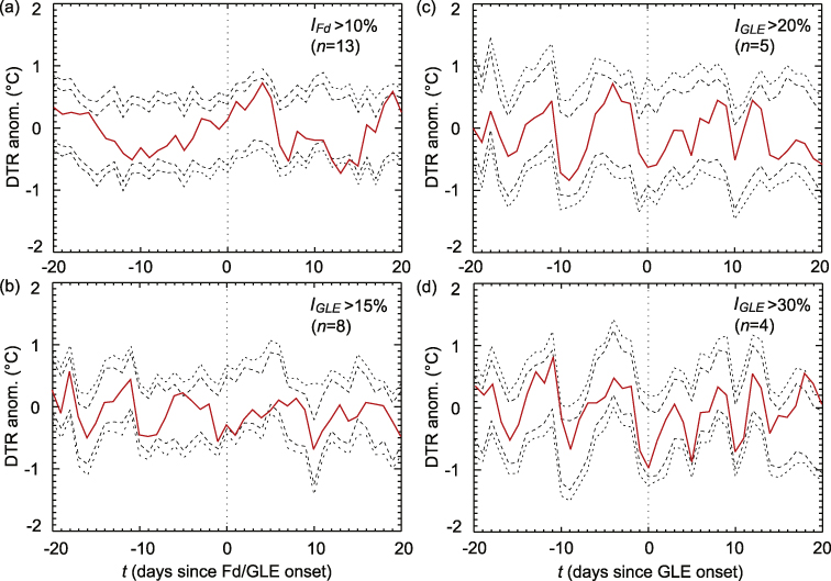
Figure 4 presents the weighted mean DTR anomaly and SE (red lines) for a t±20 day period around the onset of Fd (a)–(b) and GLE (c)–(f) events. Two-tailed p0.05 and p0.01 confidence intervals (CIs) calculated from the method described in section 2.5 are indicated with black dashed and dotted lines respectively. To test if there is a stronger response in clouds with stronger CR changes as proposed by Dragić et al (2011, 2013) several different composites have been created which isolate progressively higher magnitude NM deviations: we will refer to the magnitude of these deviations as the intensity of Fd or GLE events, denoted as IFd and IGLE respectively. Specifically, these composites are divided into samples of: IFd > 7% (n = 34, figure 4(a)), IFd > 10% (n = 13, figure 4(b)), IGLE > 10% (n = 12, figure 4(c)), IGLE > 15% (n = 8, figure 4(d)), IGLE > 20% (n = 5, figure 4(e)), and IGLE > 30% (n = 4, figure 4(f)).

Figure 4. Mean DTR anomalies and their standard errors (±1SE, red dotted lines) for a t±20 period around the onset of Fd ((a)–(b)) and GLE ((c)–(f)) events categorized by intensity. Two-tailed p0.05/p0.01 confidence intervals are presented (dashed/dotted lines) from MC-generated PDFs using 10 000 simulations at each time point t.
Download figure:
Standard image High-resolution imageFor the IFd > 7% events (n = 34), the largest (absolute) DTR deviation is observed at t+4, with an intensity of +0.30 ± 0.17 ° C (p0.07). The magnitude of these anomalies and their statistical significance is found to increase when the Fd events are restricted to relatively higher magnitude deviations (IFd > 10%,n = 13) to +0.74 ± 0.19 ° C (p0.01), as reported by Dragić et al (2011, 2013) and also by Laken et al (2012a) and Erlykin and Wolfendale (2013). We shall return to a detailed discussion of this phenomenon in section 3.2. It should also be remarked that the DTR deviations observed following Fd events are not unusual when examined over a broad time window around t0 (e.g. ±40 days), with variations of comparable or larger sizes to those around the key date observed randomly throughout the composites, as was also reported by Laken et al (2012a) and Erlykin and Wolfendale (2013).
Composites centered around GLE events for intensities (IGLE) of >10%, > 15%, > 20%, and >30% are also presented (figures 4(c)–(e)). Contrary to the report of Dragić et al (2013) no statistically significant (p ≤ 0.05) mean DTR values were observed around t0 in these composites. There was one instance where a significant reduction in DTR was identified in a GLE composite, this occurred in the IGLE > 10% sample (n = 12) shown in figure 4(c), at t+10 (−0.80 ± 0.25 p0.02). However, rather than increase in magnitude and statistical significance in the later, more intense composites (of figures 4(d)–(f)), the opposite occurs and the statistical significance is lost. This suggests that the statistical significance was merely related to the false discovery rate (FDR).
We also remark that figure 4 also clearly shows how the number of events selected for analysis influences the noise content of the composites. This phenomenon is discussed in detail in Laken and Čalogović (2013) who show that noise increases following a power-law as the sample size of composites is progressively reduced. For the n = 35 sample of figure 4(a) the average p0.05 confidence interval (CI) range was −0.41–0.32, however, as the sample size decreased to n = 4 in figure 4(f), the CI range increased considerably (−1.09–1.03). In essence, this observation tells us that as the sample size (n) is reduced, relatively higher magnitude deviations should be expected by chance. With regards to the asymmetry of the quoted CI ranges we note that this is a normal feature in geophysical data, and is the reason why CIs should be identified independently for each distribution tail as opposed to being calculated from corresponding σ values.
3.2. Composites from subpopulations
We shall now consider the increase in the amplitude and apparent significance of the DTR at t+4 that was found to occur when Fd samples were restricted by intensity to IFd > 10% (figure 5(b)). This increase results from effects of sub-sampling and not from a physical relationship between the DTR and CR flux, as we will now describe.
Figure 5. Mean DTR anomalies for Fd (a) and GLE ((b)–(d)) composites the same as figure 4 with the exception that the p0.05/p0.01 confidence intervals (CIs) are now calculated from subpopulations of 1000 MC samples. The randomly generated MC samples had a composite mean at t equivalent (within two significant digits) to their respective parent samples (see section 3.2 for further explanation). The ±1SE range around the mean is not shown in this instance for clarity, but it is identical to the relevant composites of figure 4 (as only the CIs have changed).
Download figure:
Standard image High-resolution image
The occurrence of Fd events are quasi-random with respect to the Earth's atmosphere; we note they are quasi-random instead of truly random as the Fd and GLE events occur more frequently during periods of high solar activity. Despite this, we may effectively estimate the p-value of unrestricted and weakly restricted Fd and GLE composites using samples drawn randomly from the DTR anomaly time series (which we shall refer to as the parent data). By unrestricted, we mean that no further sample restrictions have been placed on the composite event selection beyond the requirement that they are a Fd or GLE event. By adding a further selection criteria (i.e. sample restriction), such as the requirement that the intensity of the Fd events be at least >10%, we have altered the hypothesis test that must be applied and the MC technique that must be used to determine statistical significance. Of course this explanation is over-simplified, as even our parent samples (IFd > 7% and IGLE > 10%) have still been restricted (by magnitude and by occurrence within a ±7-day period of other events). As the amount of restrictions placed on the event selection increases and sample size decreases there is a progressively higher chance that standard MC-significance testing will become inadequate to properly estimate the p-value of the composite mean. However, for samples with minimal restrictions the assumption that the p-value may be accurately estimated randomly from the parent data is still valid.
For unrestricted samples the nature of the hypothesis test is encompassed by the question: is the composite mean at a given t statistically unusual with respect to random samples from the parent dataset? However, for restricted samples (i.e. subpopulations), the hypothesis test becomes: is the composite mean of a subpopulation at a given t statistically unusual with respect to other random subpopulations derived from composites with a specific mean? Consequently, to accurately estimate the probability of randomly obtaining the peak DTR changes at t+4 in the IFd > 10% sample using the MC methodology, we must do the following: the first step is to randomly select dates to create composites of n = 34 events until a composite with a mean equal to the t+4 mean of the IFd > 7% (n = 34 events) composite is achieved. From these random dates we then create a subpopulation of n = 13 events, and calculate the composite mean. This procedure is repeated and the results are accumulated to calculate a PDF, ensuring that the samples of randomly selected dates do not reoccur. The PDF is then used to calculate the p-value of the t+4 deviations. This procedure must be repeated individually for each time point t of the composite, as in each instance the hypothesis test is concerned with the probability of achieving a specific subpopulation composite mean following a specific starting point.
Essentially, we are stating that if a randomly generated composite sample does not represent the distribution of a parent dataset, then the significance of a subpopulation from the aforementioned sample cannot be evaluated from random samples of the parent dataset, but instead must be evaluated from samples that share a similar distribution (Laken and Čalogović 2013). This modified version of the MC test was applied in this work to the restricted samples, and the results are presented in figure 5. Following this, the statistical significance of the DTR anomalies at t+4 during the IFd > 10% sample are found to be non-significant (p0.07, figure 5(a)). As before, no statistically unusual variations were observed over the GLE samples (figures 5(b)–(d)).
4. Conclusions
It has been suggested that the DTR provides a useful proxy dataset to test a proposed cosmic ray (CR)–cloud link free from the limitations affecting the satellite cloud observations. Despite this advantage and the relatively long (>60 year) time span of the DTR data, we find no evidence to support previous claims of a CR–cloud link. By using significance testing with a slightly altered Monte Carlo approach to account for the effects of sub-sampling we show that earlier reports of a significant DTR increase occurring several days after Fd events noted by Dragić et al (2011, 2013), Laken et al (2012a) and Erlykin and Wolfendale (2013) resulted from an incorrect estimation of statistical significance connected with the effects of generating subpopulations. The observed increase in the amplitude of DTR anomalies following high-magnitude Fd events (IFd > 10%) are a result of stochastic variability (meteorological noise) due to the smaller number of events in restricted composites, and the appearance of statistical significance was an artifact related to sub-sampling. However, the absence of a significant response in DTR during GLE events could also be a consequence of the rather weak ionization increases during the GLE events as indicated by Usoskin et al (2011).
We conclude that there has been no evidence yet presented of a DTR response to either Fd or GLE disturbances regardless of the intensity of the disturbances, and no cosmic ray signal has thus far been identified in DTR data. We note that these results do not disprove the possible existence of a solar-related DTR response from a hypothesized CR–cloud link, rather they provide further confirmation of the results of Laken et al (2012a) that if a solar response is present in the DTR data it is too small to be clearly detectable, and by extension this indicates that if a CR–cloud link exists it has a negligible impact on climate over the timescales investigated in this analysis.
Acknowledgments
We kindly thank Alexander Dragić (University of Belgrade) and colleagues for stimulating research interest in this area. We also thank Beatriz González Merino (Instituto de Astrofísica de Canarias) and two anonymous reviewers for comments, and we gratefully acknowledge the support of the European COST Action ES1005 (TOSCA). Meteorological station data were obtained from the World Data Center for Meteorology, Asheville, USA, maintained by NOAA www.ncdc.noaa.gov/cdo-web/datasets. GLE events detected by Oulu NM obtained from Sodankyla Geophysical Observatory at www.cosmicrays.oulu.fi. Fd events detected by Mt. Washington NM obtained from NOAA/NESDIS/NGDC www.ngdc.noaa.gov/stp/solar/cosmic.htm.
Appendix.: Table of dates and magnitudes of Fd/GLE events
Table A.1. Dates and magnitudes of Fd/GLE events. *Denotes dates with insufficient data to calculate a daily mean DTR value (≤50 meteorological stations) not included in the analysis.
| Date (dd/mm/yyyy) | Type (Fd/GLE) | Abs. Mag. (%) |
|---|---|---|
| 08/01/1956 | Fd | 13.0 |
| 08/11/1956 | Fd | 7.5 |
| 21/01/1957 | Fd | 15.3 |
| 10/03/1957 | Fd | 8.2 |
| 15/04/1957 | Fd | 9.4 |
| 29/08/1957 | Fd | 13.7 |
| 23/10/1957 | Fd | 9.3 |
| 23/11/1957 | Fd | 8.5 |
| 26/03/1958 | Fd | 7.6 |
| 13/02/1959 | Fd | 8.4 |
| 12/05/1959 | Fd | 12.8 |
| 30/03/1960 | Fd | 10.6 |
| 16/11/1960 | Fd | 14.2 |
| 28/01/1967 | GLE | 17.0 |
| 26/05/1967 | Fd | 7.5 |
| 28/10/1968 | Fd | 11.1 |
| 24/01/1971 | GLE | 16.0 |
| 01/09/1971* | GLE | 14.0 |
| 31/10/1972* | Fd | 7.8 |
| 30/03/1976 | Fd | 7.6 |
| 22/11/1977 | GLE | 13.0 |
| 14/02/1978 | Fd | 12.6 |
| 06/03/1978 | Fd | 7.4 |
| 07/05/1978 | GLE | 84.0 |
| 13/07/1978 | Fd | 7.2 |
| 26/08/1978 | Fd | 7.2 |
| 07/07/1979 | Fd | 7.8 |
| 06/06/1980 | Fd | 7.4 |
| 30/11/1980 | Fd | 8.3 |
| 24/02/1981 | Fd | 11.3 |
| 23/07/1981 | Fd | 9.1 |
| 12/10/1981 | GLE | 11.0 |
| 30/01/1982 | Fd | 8.0 |
| 06/06/1982 | Fd | 9.7 |
| 10/07/1982 | Fd | 25.0 |
| 18/09/1982 | Fd | 9.0 |
| 07/12/1982 | GLE | 26.0 |
| 16/02/1984 | GLE | 15.0 |
| 06/02/1986 | Fd | 9.8 |
| 12/03/1989 | Fd | 15.5 |
| 16/08/1989 | GLE | 12.0 |
| 29/09/1989 | GLE | 174.0 |
| 28/11/1989 | Fd | 16.0 |
| 07/04/1990 | Fd | 7.7 |
| 24/03/1991 | Fd | 23.5 |
| 06/11/1997 | GLE | 11.0 |
| 14/07/2000 | GLE | 30.0 |
| 13/12/2006 | GLE | 92.0 |