
Abstract
Data from a 500-year preindustrial control run of climate model INMCM4 show distinct climate variability in the Arctic and North Atlantic with a period of 35–50 years. The variability can be seen as anomalies of upper ocean density that appear in the Arctic and propagate to the North Atlantic. The density gradient in a northeast–southwest direction alternates with the density gradient in a northwest–southeast direction. A positive density anomaly in the Arctic is associated with a positive salinity anomaly, a positive surface temperature anomaly and a reduction of sea ice in the Barents and Kara Seas. The nature of the variability is a vertical advection of density by thermal currents similar to that proposed in Dijkstra et al (2008 Phil. Trans. R. Soc. A 366). The cycle of model variability shows that after a negative anomaly of density in the northwest Atlantic, one should expect warming in the Arctic in 5–10 years. The ensemble of decadal predictions with climate model INMCM4 starting from 1995 shows that warming in the western Arctic and especially in the Barents Sea observed in 1996–2010 can be reproduced by eight of ten ensemble members. Arctic climate predictability in this case is associated with a proposed mechanism of a 35–50 year North Atlantic–Arctic oscillation.
Export citation and abstract BibTeX RIS

Content from this work may be used under the terms of the Creative Commons Attribution 3.0 licence. Any further distribution of this work must maintain attribution to the author(s) and the title of the work, journal citation and DOI.
1. Introduction
In spite of significant progress in understanding many climatic and weather phenomena, the mechanism of multidecadal natural climate variability in the Arctic and North Atlantic is still under discussion. Several mechanisms associated with the oscillation of Atlantic overturning circulation have been proposed. In Delworth et al (1993) in the coupled atmosphere–ocean model, irregular oscillations in the North Atlantic were found with a time scale of about 50 years. The mechanism is the change of overturning circulation because of the change of water density in the sinking region. The reason for the fluctuations of density is the change of the overturning circulation itself as well as an associated change of gyre circulation. Griffies and Tzipermann (1995) in a simple four-box model found a damped oscillatory mode that can produce oscillations with a period of about 50 years. The mechanism is delayed feedback between the overturning circulation and northward transport of temperature and salinity by the overturning circulation. The mechanism in the four-box model looks similar to that found in the full model in Delworth et al (1993). In Griffies and Tzipermann as well as in Delworth and Greatbatch (2000) it was shown that stochastic atmospheric forcing is responsible for excitation of the oceanic oscillatory mode. In Timmermann et al (1998) the proposed mechanism for the 35-year oscillation in the North Atlantic was also oscillation of overturning circulation, but the interaction of the oceanic mode with the North Atlantic oscillation (NAO) is crucial. Enhancement of overturning circulation produces a warm anomaly in the North Atlantic that produces a positive NAO index and an increase of Ekman transport of fresh water from the northwest to the sinking region, which leads to a decrease of density and a decrease of overturning circulation. Jungclaus et al (2005) found that oscillation of overturning circulation and deep convection in deep water formation regions modulates the export of fresh water from the central Arctic to the North Atlantic, and it seems to be an additional mechanism of the oscillation. In Latif et al (2007) it is shown using observational data that oscillation of the Atlantic meridional circulation is probably responsible for sea surface temperature (SST) fluctuations. von der Heydt and Dijkstra (2007) show that in an idealized two-basin model with Pacific and Atlantic oceans maximum multidecadal variability is concentrated in the region of deep water formation. In other studies oscillation of overturning circulation is not the primary reason for multidecadal oscillation in the North Atlantic. Dijkstra et al (2008) show using eigenmodes of linearized simplified equations of Atlantic oceanic dynamics that a 'thermal Rossby wave' is the mechanism of the oscillation and westward propagation of SST anomalies in the North Atlantic. A similar study for the Arctic Ocean (Frankcombe and Dijkstra 2010) proposed a mechanism of a 'saline Rossby wave' for multidecadal variability in an idealized model of the Arctic. The authors of the last study, as well as Frankcombe and Dijkstra (2011), show that multidecadal variability in the Arctic in climate model GFDL CM2.1 can also probably be explained by the mechanism of a 'saline Rossby wave'. Two periods of multidecadal variability in North Atlantic in GFDL CM2.1 are explained by a 'thermal Rossby wave' in the Atlantic and the influence of a 'saline Rossby wave' from the Arctic (Frankcombe and Dijkstra 2011). Recent studies of decadal potential predictability (Branstator et al 2012) and actual decadal predictability (Bellucci et al 2013) show that in the North Atlantic and Arctic the climatic system has the longest memory of the initial conditions. The aim of this paper is to study the mechanism of multidecadal variability in the Arctic and North Atlantic in climate model INMCM4. An attempt to predict the phase of the studied oscillation in 1996–2010 using the initial oceanic condition of 1995 with an ensemble of model runs is also considered.
2. Model, data and methods
To study multidecadal variability in the Arctic and North Atlantic, data from a 500-year preindustrial run with climate model INMCM4 were used. The model contains an atmospheric block with a resolution of 2° × 1.5° in longitude and latitude and 21 vertical levels, and an oceanic block with a resolution of 1° × 0.5° in longitude and latitude and 40 vertical sigma levels. Flux adjustment in the coupling of atmosphere and ocean is not applied. A model description and analysis of a present day model climate can be found in Volodin et al (2010).
Multidecadal variability was studied on the basis of five-year mean model data. A parabolic trend was removed from the data. Composites of different variables for different phases of North Atlantic–Arctic multidecadal oscillation were calculated as follows. Empirical orthogonal functions (EOFs) of global near-surface temperature were calculated. The first EOF (22% of variance) is localized in the Arctic, with maxima in the Central Arctic, Barents and Kara Seas (figure 1), where the correlation of expansion coefficient with temperature exceeds 0.8. The spectrum of the expansion coefficient of the first EOF shows significant peaks at periods of 35–50 years. The composite for year 0 was calculated as a mean anomaly for five-year time intervals, when the expansion coefficient of the first EOF increased. That means that the increment of the coefficient (the value five years after minus the value the years before) was above the mean time plus one standard deviation. The composite for year −5 was calculated as a mean anomaly for five-year time intervals just before that used for the calculation of the composite for year 0. The composite for year −10 is the mean anomaly for five-year time intervals 10 years before five-year intervals when the expansion coefficient increased. Similarly, composites for year 5 and year 10 were calculated. In general, composites for years from −10 to 10 show evolution of the selected variable during approximately a half-period of the oscillation, from negative to positive phase.
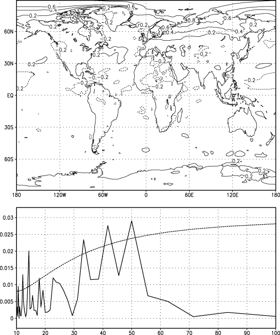
Figure 1. Correlation of the expansion coefficient of EOF-1 with a five-year mean near-surface temperature (top) and the spectrum of the expansion coefficient, K (bottom). The dashed line represents the significance level of spectral peaks at 99%.
Download figure:
Standard image High-resolution imageAn attempt to predict multidecadal Arctic and North Atlantic variability was made in the following way. The initial state of the ocean was prescribed as the sum of the mean model state for the beginning of January in the preindustrial run plus the anomaly for January 1995. The anomaly for January 1995 was calculated using monthly mean data of a simple ocean data assimilation (SODA), Carton and Giese (2008). The anomaly of January 1995 was calculated with respect to January of 1979–2008. Anomalies of temperature and salinity were only added to model preindustrial climatology. The initial state of other prognostic oceanic variables (U and V currents, sea surface height, sea ice parameters) were prescribed as the model climatological mean for preindustrial January, assuming that currents and sea surface height adjust quickly towards geostrophical balance with temperature and salinity. A simple linear interpolation from the grid of SODA (0.5° × 0.5° in longitude and latitude, 40 z-levels) to the model grid was utilized. The initial atmospheric state was taken from the preindustrial run (data for the beginning of January) and did not correspond to any observed initial state. Such initialization assumes that most of the useful information for prediction is concentrated in ocean temperature and salinity. Initialization of anomalies with respect to model climatology rather than total temperature and salinity from SODA allows us to avoid model drift towards model climate during the forecast period. An ensemble of ten predictions was performed. To obtain different members of the ensemble, small changes were brought into the initial data. The duration of each run was equal to 30 years, but we discuss here the prediction for years 1996–2010. No changes of external forcings, including concentration of greenhouse gases, aerosols or solar radiation flux were taken into account in the prediction ensemble. Therefore, only natural variability rather than signals from global warming can be reproduced in the considered prediction. The predicted anomaly of the chosen variable was calculated as the difference of data in the ensemble for the appropriate years minus data of the preindustrial run. It is compared with the anomaly from NCEP (Kalnay et al 1996) and MERRA (Rienecker et al 2011) reanalysed for years 1996–2010 with respect to years 1979–2010.
3. Results
The evolution of the model for the North Atlantic–Arctic oscillation from negative to positive phase is presented by composites of surface ocean density for years −10, −5, 0, 5, 10 (figure 2). In year −10 one can see a negative anomaly over most of the Arctic, while a positive anomaly is located in the North Atlantic. In year −10 we have a northeast–southwest gradient of surface density. In year −5 the anomaly of density in the Arctic starts to decrease in magnitude and move to the southwest, towards the east coast of Greenland. In year 0 one can see a northwest–southeast density gradient with negative anomaly near the east coast of Greenland and a positive anomaly near the west coast of Europe. The anomaly in the Arctic becomes small. During the next 10 years again the northeast–southwest gradient of density increases, but with sign opposite to that in year −10. We have a positive anomaly in Arctic and a negative anomaly in the North Atlantic. Anomalies of density in the considered region are defined generally by anomalies of salinity rather than temperature. In general anomalies of temperature have the same sign as anomalies of density (figure 2) and this should produce the opposite effect on density, but the impact of salinity is stronger. Oscillation of density produces oscillation of deep convection in Labrador, Greenland, Irminger and Norwegian Seas as well as oscillation of the Atlantic overturning circulation. Atlantic overturning circulation is defined as the meridional streamfunction maximum at 25–35 N, 1000–2000 m depth and it has a minimum in year 5, approximately 5 years after the minimum of surface density in sinking regions. The time spectrum of meridional overturning circulation has a distinct maximum at 35–50 years (not shown) as well as that for the expansion coefficient of the first EOF of surface temperature. There is a relation between North Atlantic–Arctic oscillation and NAO (negative NAO phase occurs in years −10 to −5), but only a small part of the total multidecadal variability of the NAO index can be explained in such a way. There is no significant peak in the NAO spectrum at 35–50 years (not shown).
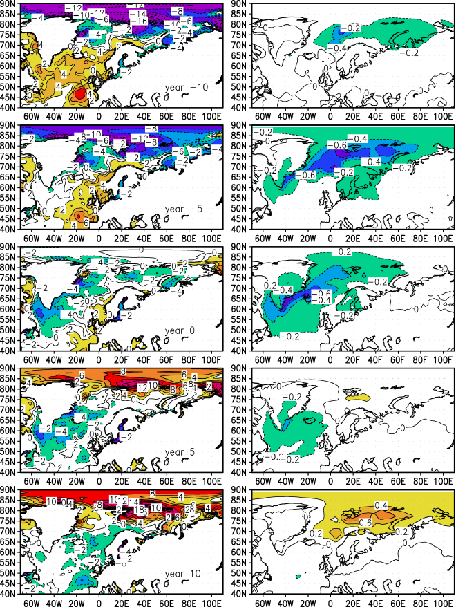
Figure 2. A composite of the anomalies of surface density 10−2 kg m−3 (left) and near-surface air temperature, K (right), for year −10, −5, 0, 5 and 10.
Download figure:
Standard image High-resolution imageOf course, it is very difficult to prove accurately that in model any chosen mechanism is the reason for the considered oscillation. Nevertheless, we suppose that the mechanism of westward propagation of density anomalies is similar to that proposed in Dijkstra et al (2008), but in our case salinity rather than temperature is responsible for the density anomaly and thermal current. Figure 3 shows the mechanism of propagation of the density anomaly along the basin. Axis X corresponds to longitude, axis Y—latitude, axis Z—height. Initially we have a negative density anomaly along the northern wall of the basin. Just southward of the negative anomaly of density we have a vertical shift of zonal current UX according to the equation of thermal wind:
where g is the acceleration due to gravity, ρ0 the mean water density, f the Coriolis parameter and ρ' the density anomaly. The presented thermal current upwelling is located near the eastern boundary and the downwelling is placed near the western boundary of the basin. For a stable condition, the potential density has to increase with depth, so upwelling leads to advection of high density producing a positive density anomaly, while downwelling leads to advection of low density and produces a negative density anomaly. After time τ one can expect a negative density anomaly near the western boundary and a positive density anomaly near the eastern boundary. Then, repeating our reasoning, after one more time interval τ we will have a positive anomaly of density near the northern boundary and a negative density anomaly near the southern boundary, which is opposite to the initial condition. Here time interval τ is a quarter of a period of oscillation. We can estimate it in the following way. If we assume that the spatial scale of density anomaly in directions X,Y,Z is Δx,Δy and Δz, then according to the contiguity equation, vertical current UZ near the northern boundary and near the western and eastern boundaries is:
and the tendency of density induced by vertical advection is:
where ∂ρ0/∂z is the vertical gradient of the potential density. We can estimate τ as time when the density anomaly due to vertical advection near the western or eastern boundary will be of the same magnitude as the initial anomaly near the northern boundary:
Substituting numerical values of variables typical for the model climate in the North Atlantic–Arctic region Δx = 3 × 10⁶ m,Δy = 106 m,Δz = 100 m,∂ρ0/∂z = 5 × 10⁻³ kg m−4,f = 6 × 10⁻⁵ s−1,g = 10 m s−2 one can find an estimation of a quarter of period τ ≈ 11 years. This corresponds with a period of 35–50 years that was found in the model. The values of Δx,Δy,Δz were chosen as a typical scale of the anomalies of density in longitude, latitude and height. Scales Δx,Δy can be estimated from figure 2; vertical scale Δz was chosen as 100 m, because the typical thickness of anomalies of density associated with North Atlantic–Arctic oscillation in the model is just 100 m.

Figure 3. Scheme of anomalies of density, thermal current, upwelling, downwelling and tendency of density in multidecadal oscillation. The figure is similar to figure 5 in Dijkstra et al (2008) but with anomaly of density rather than temperature.
Download figure:
Standard image High-resolution imageFigure 4 shows the composites of the difference between currents at 0 and 100 m for year −10 and year 0. The presented currents correspond with thermal current relationship (1) and density anomalies for the appropriate year (figure 2). In year −10, currents are directed mainly from southeast to northwest, along lines of constant ρ'. Such currents induce downwelling with advection of low density from the upper layers near the east coast of Greenland, and upwelling with advection of high density from deep layers near the west coast of Europe. In year 0 in Greenland, Norwegian and Irminger Seas the currents are directed from northeast to southwest along lines of constant density. Such currents induce upwelling and an increase in surface density in the Arctic and downwelling and a decrease of upper layer density in the North Atlantic.
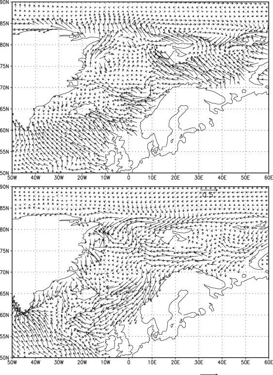
Figure 4. A composite of the difference of ocean current anomalies, cm s−1 at 0 and 100 m for year −10 (top) and year 0 (bottom).
Download figure:
Standard image High-resolution imageOscillation of Atlantic overturning streamfunction can probably only play a secondary role in the mechanism, because density fluxes generated by it are about one order below that generated by the oscillation of currents derived by the thermal wind relation. Also interaction with NAO probably does not play such an important role in the mechanism, as in Timmermann et al (1998), because the minimum of the NAO index in this study happens a quarter of period earlier than the minimum of temperature in the North Atlantic, while in Timmermann et al (1998) both minima coincide.
It would be interesting to test whether such a mechanism could have contributed to the recent warming in the Arctic that has been observed in the last 10–15 years. Of course, global warming is one of the main reasons for recent Arctic warming, but the impact of natural variability could also be significant. To test this assumption, an ensemble of decadal prediction was performed with climate model INMCM4. The methodology and the choice of initial data have been described in section 2. Assuming the period of model oscillation as 35–50 years, the characteristic life time of positive or negative anomalies in the Arctic can be estimated as 1/3 of a period or approximately 15 years. Such 15 year averaging should be the most useful for the prediction of climate anomalies associated with model North Atlantic–Arctic oscillation. So, if one intends to predict the climate anomaly in the Arctic in the last 15 years (1996–2010), one should take the initial condition just before this time interval. The initial anomaly of surface density can be seen in figure 5. A negative anomaly in the northwest Atlantic and a positive anomaly to the north of 82 N produce an anomaly similar to a linear combination of that presented in figure 2 for year 0 and year 5. The anomaly that one can expect in 1996–2010 will be a linear combination of anomalies in years 5, 10 and 15. The anomaly for year 15 is not presented, but it looks similar to that for year −5 with the opposite sign. Therefore, in 1996–2010 we should expect a positive density anomaly in the Arctic and a positive temperature anomaly with a maximum in the Barents, Kara and Norwegian Seas. The ensemble of decadal predictions shows that this is indeed the case. Eight of ten members show warming with maxima in the Barents, Kara and Norwegian Seas, and only two remaining members show cooling. The near-surface temperature anomaly averaged over ten members (figure 6) shows warming up to 0.8 K in the Barents Sea which is significant at the 99% level. Root mean square deviation of individual members is also a maximum in Barents and Kara Seas (0.6 K). NCEP and MERRA reanalyses also show a positive temperature anomaly in 1996–2010 with a maximum in the Barents Sea. An ensemble of predictions underestimates the value of warming by a factor of 1.5–2 and is not capable of reproducing some warming in the whole Arctic as well as over Eurasia, but the reason is probably a fixed greenhouse gas concentration in the ensemble of predictions.
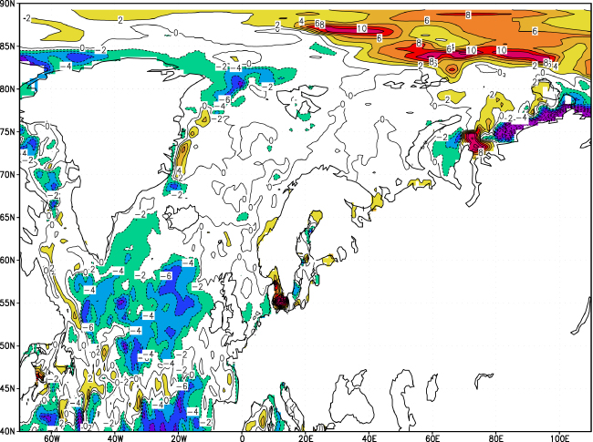
Figure 5. Anomaly of surface density 10−2 kg m−3 in January 1995 with respect to January 1979–2008 in SODA.
Download figure:
Standard image High-resolution image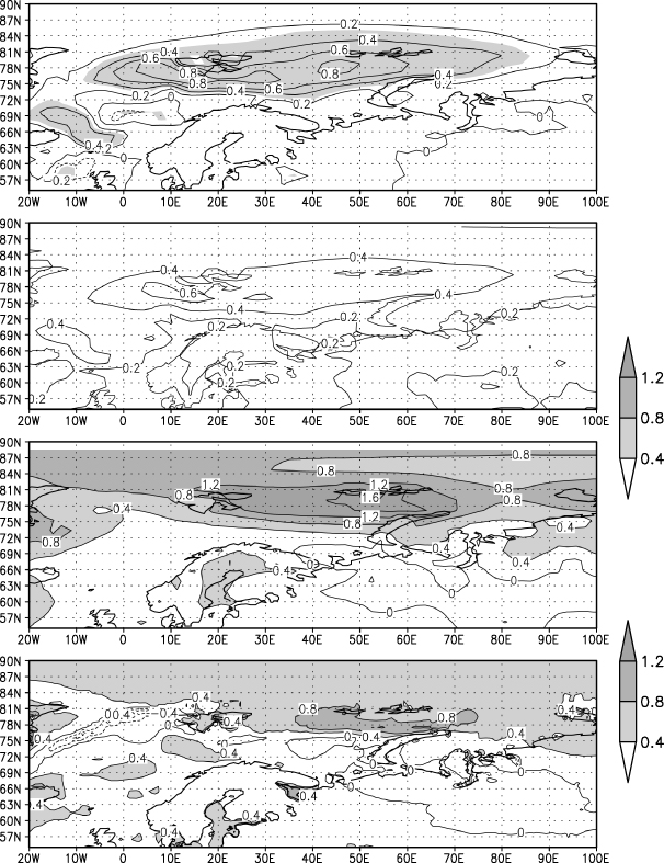
Figure 6. Top to bottom: anomalies of near-surface temperature in 1996–2010 in the ensemble of model runs, shading means statistical significance at the 99% level according to the t-test; root mean square deviation of ensemble members; anomaly of near-surface temperatures in 1996–2010 with respect to 1979–2010 in NCEP reanalysis; as above, but for MERRA reanalysis.
Download figure:
Standard image High-resolution image
4. Summary
In the preindustrial run performed with climate model INMCM4 multidecadal variability in the Arctic and North Atlantic shows significant peaks at periods of 35–50 years. During a quarter period, a negative density anomaly in the Arctic and a positive density anomaly in the North Atlantic (northeast–southwest gradient) is changed to a negative density anomaly near the east coast of Greenland and a positive density anomaly near the west coast of Europe (northwest–southeast gradient). Then, after another quarter period, one can see a positive density anomaly in the Arctic and a negative density anomaly in the Atlantic, i.e. the pattern is opposite to the initial one. The proposed mechanism of the oscillation is similar to that discussed in Dijkstra et al (2008). A thermal current induced by the density gradient is responsible for upwelling and downwelling, and vertical advection produces new surface anomalies in the density. Several studies (Delworth et al 1993, Timmermann et al 1998, Griffies and Tzipermann 1995, and others) propose mechanisms of multidecadal North Atlantic–Arctic oscillation in the climate model as the effect of oscillations in the Atlantic overturning circulation. However, this is not the case for the present study, where oscillation of overturning circulation probably plays a secondary role. The difference in the mechanism leads to a difference in the form of the oscillation. One can see a clear propagation of the density anomaly from the Arctic to the North Atlantic in the present study, while there is no clear propagation in the studies mentioned above. Ensemble of decadal predictions show that approximately half of the warming in the Arctic, with a maximum in the Barents Sea, observed in 1996–2010 can be reproduced as an ensemble mean anomaly of the forecasts of natural variability started in 1995. The remaining increase of temperature can probably be associated with global warming.
Acknowledgments
This study was supported by the Russian Fund for Basic Research, grant 12-05-00556a, and the Ministry of Education and Science RF, grants 2012-1.1-12-000-1007-013 and 2012-1.2.1-12-000-1008-009.