
Abstract
Bioenergy has the unique potential to provide a dispatchable and carbon-negative component to renewable energy portfolios. However, the sustainability, spatial distribution, and capacity for bioenergy are critically dependent on highly uncertain land-use impacts of biomass agriculture. Biomass cultivation on abandoned agriculture lands is thought to reduce land-use impacts relative to biomass production on currently used croplands. While coarse global estimates of abandoned agriculture lands have been used for large-scale bioenergy assessments, more practical technological and policy applications will require regional, high-resolution information on land availability. Here, we present US county-level estimates of the magnitude and distribution of abandoned cropland and potential bioenergy production on this land using remote sensing data, agriculture inventories, and land-use modeling. These abandoned land estimates are 61% larger than previous estimates for the US, mainly due to the coarse resolution of data applied in previous studies. We apply the land availability results to consider the capacity of biomass electricity to meet the seasonal energy storage requirement in a national energy system that is dominated by wind and solar electricity production. Bioenergy from abandoned croplands can supply most of the seasonal storage needs for a range of energy production scenarios, regions, and biomass yield estimates. These data provide the basis for further down-scaling using models of spatially gridded land-use areas as well as a range of applications for the exploration of bioenergy sustainability.
Export citation and abstract BibTeX RIS

Content from this work may be used under the terms of the Creative Commons Attribution 3.0 licence. Any further distribution of this work must maintain attribution to the author(s) and the title of the work, journal citation and DOI.
1. Introduction
The production of electricity from biomass could provide a critical back-up energy source to renewable energy portfolios that are currently dominated by intermittent wind and solar energy resources [1]. The stored chemical energy in biomass can be deployed to produce electricity on demand, reducing the overall intermittency of a renewable energy portfolio. The storage capacity of biomass is particularly important for the seasonal intermittency of wind and solar energy which are not easily addressed by alternative storage schemes such as pumped hydropower, thermal energy storage, compressed air energy storage, flow batteries, fuel cells, flywheels, or superconducting magnetic energy storage [2, 3]. Seasonal variation in wind and solar energy production require much larger amounts of energy storage than required to address short-term intermittency in wind and solar energy production as well as energy storage over longer periods.
In addition to energy storage, biomass electricity has the unique potential of providing a carbon-negative and highly efficient approach to bioenergy production. Mandated reductions in carbon emissions may require technological solutions that cannot be met by carbon-neutral solutions alone. Biomass electricity can provide a carbon-negative solution when biomass cultivation and energy conversion technologies are coupled to carbon capture and sequestration technologies [4, 5]. Alternatively, there are approaches to bioenergy production that can results in large life-cycle emissions of greenhouse gases (GHG) due to fossil fuel energy consumed during the cultivation of biomass, fossil fuel energy consumed during the conversion of biomass into useful energy forms, and land-use change [6, 7]. Creating a carbon-negative approach to biomass electricity will require careful consideration of these cultivation, energy conversion, and land-use factors. Biomass electricity has also been shown to provide a highly efficient approach to providing renewable transportation energy that is complementary to existing liquid fuel approaches [8–11].
Despite the important role that bioenergy may play in future energy systems, the economic and environmental outcomes of bioenergy remain highly uncertain. This uncertainty is dominated by bioenergy land-use effects that may disrupt ecological systems and food economies but may also contribute to rural development and provide new options for enhancing soil quality, water resources, and biodiversity [4, 12–15]. Field studies suggest a path to reduce negative land-use impacts through the application of abandoned agriculture lands for biomass cultivation as opposed to prime agriculture lands [4]. A global-scale analysis of abandoned lands estimated the bioenergy potential of these lands as 32–41 EJ or 7%–8% of primary energy demand [16, 17]. While these coarse global estimates are useful for large-scale planning, more practical technological and policy applications will require regional, high-resolution information on biomass availability.
Here we present county-level estimates of the magnitude and distribution of abandoned agriculture lands in the US using remote sensing, agriculture inventories, and land-use modeling. Furthermore, we explore one potential application of these data to quantifying the seasonal energy storage that could be provided by bioenergy to compensate for the seasonal intermittency of wind and solar power. The county-level land-use data resulting from this study are extended to a gridded product in a companion paper [18]. The land-use data resulting from this analysis are available online (https://eng.ucmerced.edu/campbell/).
2. Methods for land-use availability and bioenergy potential
We employ a GIS-based modeling approach to develop maps of land availability, biomass yields, and bioenergy production with a county-level resolution for the US domain. The GIS model was developed using the ArcGIS spatial analyst extension to conduct the raster and vector calculations described below. The land-use model quantifies the spatial distribution of abandoned agriculture. Abandoned agriculture is divided into abandoned cropland and abandoned pasture. Here available abandoned agriculture lands are defined as an area of land that was once classified as cropland or pasture and is currently not classified as cropland, pasture, forestland, or urban areas. The input data for the land-use analysis is the USDA county-level cropland database which includes cropland areas for each county from the years 1850 to 1997 [19]. Between 1850 and 1940, the data are in 10-year increments. Between 1940 and 1997 the data are in 4 or 5 year increments. The abandoned cropland area for each county is the difference between maximum area over the time series for each county (years 1850–1997) and the area in the final time step (year 1997),

where Ai is the abandoned cropland areas, C is the cropland area, and i and t are the indices for county and year, respectively. Note that in equation (1), the maximum cropland areas from each county are not necessarily from the same year but may be from a range of years. The county-level cropland data had erroneous spikes [19] for less than 5% of the data which were removed prior to the analysis. Estimates of abandoned pasture land as well as estimates of areas of land that was converted from agriculture to urban or forestlands were obtained from a previous analysis [16, 17]. More recent cropland area changes after 1997 were explored using the USDA/NASS database and found to be small relative to area changes from 1850 to 1997. However, recent work presents a small but rapid expansion of cropland areas from 2006 to 2011 which suggests that our analysis may overestimate abandoned croplands in some localities [20].
The county-level data suffered from a change in land-use definitions between 1940 and 1945 which introduces an artificial decline in cropland area [19, 21]. The period of 1945–1997 has a more restrictive definition of cropland used for pasture than for the period of 1850–1940. We adjusted for the definition change by subtracting the 1940–1945 area change from the county areas for years 1850–1940.
There are several sources of uncertainty in these land availability estimates. The spatial resolution of the croplands (county-level) is not consistent with the pasture, forest, and urban land (5 min × 5 min) data. Furthermore the crop and pasture data have a different format than the forest and urban area data. The crop and pasture data are density data, providing the per cent of each pixel that is occupied by crops or pastures. Alternatively, the forest and urban data classify each pixel as entirely forest or urban or other land cover without providing the fraction of the pixel that is covered by such land cover. Validation data are not currently available for determining the magnitude of this uncertainty associated with the range of spatial resolutions and classification schemes. However, we also report abandoned cropland areas that are not combined with pasture areas and are not filtered using forest and urban areas in order to provide an upper estimate for land availability that is not associated with these uncertainties.
We compare these new abandoned cropland area estimates to previous estimates that were based on the relatively coarse data from the SAGE and HYDE global gridded databases [22, 23]. HYDE crop and pasture estimates range from 1700 to 2000 in 10-year increments. We developed HYDE-based abandoned cropland areas using only data from 1850 to 2000. Estimating abandoned cropland from HYDE using data from 1850 to 2000 yielded the same results as using data from 1700 to 2000. SAGE crop areas range from years 1700 to 1992 in 10-year increments. Abandoned crop estimates were calculated using data from 1850 to 1992.
Biomass yields and energy conversion efficiencies are based on approaches applied in previous global assessments [16, 17]. Crop yields are based on the CASA primary production model of natural vegetation and are in the range of observed yields for the candidate biomass crop switchgrass [24] but lower than the relatively sparse observations available for the candidate crop Miscanthus [25]. We used the CASA model to spatially extrapolate reported biomass yields for switchgrass and Miscanthus [25]. The ratios of the observed Miscanthus and switchgrass yields in Illinois with respect to the CASA yield simulations in Illinois were applied to the CASA yield map to provide a map of Miscanthus and switchgrass yields. The above-ground yields at the Illinois site were 29.6 t dry biomass ha−1 yr−1, 10.4 t dry biomass ha−1 y−1, and 9.9 t dry biomass ha−1 y−1 for the Miscanthus plot, switchgrass plot, and CASA grid cell, respectively. These yield estimates may provide an upper estimate of biomass yields due to the potential for soil degradation on abandoned lands.
3. Seasonal storage and demand model
Recent work by Converse considers a range of energy storage options for compensating for the seasonal-scale intermittency of wind and solar energy production [2]. This analysis considers the seasonal electricity storage requirements for a renewable electricity system that uses no fossil fuels. The seasonal energy storage requirement was based on current national wind and solar production data for the US domain. This approach is designed to assess the seasonal energy storage requirement for a future US energy scenario in which wind and solar energy are the dominant energy sources. The annual wind and solar production is assumed to be equal to the annual energy demand. Three renewable energy scenarios are examined including only wind production, only solar production, and the energy production divided evenly between wind and solar. This approach assumes that current seasonal variations of electricity demand, solar production, and wind production in the future will be similar to the current seasonal variation rather than projecting alternative seasonal capacity factors. This approach only estimates energy storage requirements at the seasonal scale and does not consider storage requirements at different timescales (e.g., diurnal storage requirements) or the potential for existing hydropower to provide storage or back-up power. Alternatively, if a larger generation capacity had been assumed then the seasonal storage requirements would be reduced.
We quantify the seasonal energy storage requirement using DOE Energy Information Administration (EIA) monthly data for current electricity demand, current wind production, and current solar production at the level of three regional power grids (east grid, Texas/ERCOT grid, and west grid) [26]. Solar energy is not analyzed for the ERCOT grid due to the relatively small scale and inconsistency of EIA data for this region. The simulated monthly storage is,

where S is the monthly storage (normalized to annual demand), D is the electricity demand (normalized to annual demand), P is the electricity production (normalized to annual production), and m represents the month. The annual seasonal storage requirement (SD) is,

The annual storage requirement is the storage capacity that would be required to offset energy deficits due to seasonal intermittency. This simple model provides an estimate of the annual storage capacity needed for storage technologies that can store excess wind and solar energy during months when wind and solar production exceed demand. When bioenergy is the back-up energy technology, the surplus wind and solar energy cannot be stored and the annual energy storage is simply the sum of the monthly deficits during months when production is less than demand.
4. Land availability results
Abandoned cropland area (not adding abandoned pasture or removing croplands converted to forest or urban areas) for the years 1850–1997 is found to be 94.5 Mha (million hectares) using the uncorrected county-level USDA cropland data. However 12 of the counties have anomalous cropland areas in which a spike appears in the timeline that is as much as seven times the total land area in a county. Removing these anomalous spikes results in 99.94% of counties having cropland areas that are less than the total county area and all counties having cropland areas that are less than 105% of total county area. The abandoned cropland estimate resulting from this revised data set is 90.9 Mha. Adjusting for the land-use definition change (1940–1945) results in an abandoned cropland area of 71 Mha or about 41% of the current cropland area (figure 1). There is only a 2% difference in the estimated area if the 1940–1945 data gap is filled using one time step before and after the gap or two time steps before and after the gap.
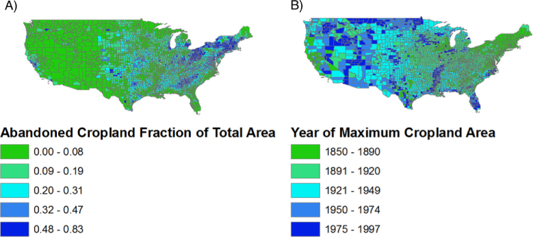
Figure 1. Abandoned cropland (A) and year of maximum cropland area (B). Abandoned cropland areas are presented as the fraction of county area and are total abandoned areas not excluding conversion to forest or urban areas.
Download figure:
Standard image High-resolution imageOur abandoned cropland area estimate of 71 Mha is larger than previous estimates that were based on coarse global data sets (figure 2). We used a similar land-use modeling approach with the SAGE global gridded databases which result in 44 Mha of abandoned cropland. These global gridded databases were derived from state-level rather than county-level census data. Our county-level results may be larger than previous state-level results because of aggregation effects in the state-level results. To quantify this source of error we aggregated the county-level data to the state-level and repeated the analysis which resulted in a greater similarity to the SAGE areas (figure 2). The aggregation effect is small in the northeast relative to other regions of the US, perhaps due to the smaller size of the states in this region. One possible driver of this aggregation effect is that counties with cropland abandonment may be masked by counties with cropland area growth when both exist within the same state. If aggregation effects are also occurring at the county-level then our county-level results may also underestimate the magnitude of the abandoned areas.
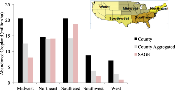
Figure 2. Regional abandoned cropland areas based on county-level data, county-level data aggregated to the state-level, and previous global study based on state-level data (SAGE).
Download figure:
Standard image High-resolution imageThe timing of cropland abandonment is related to the year of maximum crop area which is on average 1933 (±38) for the US domain (figure 1(B)). Restricting the land-use analysis to the years 1900–1997 results in 93% of the abandoned area estimate as opposed to using the entire data set for years 1850–1997 (figure 3).
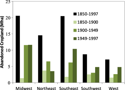
Figure 3. Abandoned cropland areas based on temporal subsets of the data spanning year 1850–1900, 1900–1949, and 1949–1997.
Download figure:
Standard image High-resolution imageThe abandoned agriculture area accounting for cropland abandonment, pasture abandonment, and excluding conversion of these lands to forest or urban areas are plotted in figure 4. The total abandoned agriculture is 99 Mha, which is considerably larger than the US results using global data of 51–67 Mha [16].

Figure 4. Total abandoned agriculture as a per cent of county area. Abandoned agriculture includes abandoned cropland and abandoned pasture but excludes abandoned lands that have been converted to forests or urban areas.
Download figure:
Standard image High-resolution image5. Seasonal energy storage results
The monthly time series for energy demand, wind energy, and solar energy are plotted in figure 5. The seasonal amplitude of solar energy is considerably larger than the seasonal amplitude of wind energy and energy demand. While the amplitude of the wind energy is relatively low, the wind variation is not in phase with the demand variation.

Figure 5. Monthly wind electricity production, solar electricity production and electricity demand as a percentage of the annual totals for each. Seasonal energy profiles for states within the (a) Western electric grid, (b) Eastern electric grid and (c) ERCOT (Texas) electric grid.
Download figure:
Standard image High-resolution imageThe required seasonal storage requirement is plotted as a fraction of the total electricity demand in figure 6. The required storage varies from 7% to 26% of annual electricity demand suggesting that seasonal storage would be an important component of a renewable energy system based on wind and solar. Because of the relatively low seasonal variability of wind energy, it follows that required seasonal storage by the wind energy scenario is low relative to the solar scenario while the wind and solar mixed scenario falls in between. Our results have a similar overall range as previous results based on national-scale data [2], but differ in terms of the storage required for each specific pathway and add a regional component to the analysis.

Figure 6. Seasonal electricity storage required for Western electric grid, Eastern electric grid and ERCOT (Texas) electric grid based on an energy production system that is entirely wind, entirely solar, or a 50% mix of wind and solar.
Download figure:
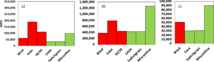
Standard image High-resolution imageThe capacity of biomass to meet the seasonal storage requirement is plotted for a range of biomass feedstocks, energy production scenarios, and regions in figure 7. In the estimates shown in figure 7, the biomass energy values represent biomass energy that can be potentially obtained from available abandoned cropland (not including abandoned pasture) within the respective region. Bioenergy can meet more than half of the storage requirements for most cases considered if all the available biomass grown on abandoned croplands is utilized. Bioenergy can meet all of the seasonal storage requirements for the 100% solar production scenario only for the most optimistic assumption regarding biomass crop yields.
Figure 7. Annual electricity energy storage deficit and bioenergy availability for a range of biomass feedstock crops. Storage needs by resource are in red (if 100% of the annual demand was met only by the specified resource) and estimates of available energy from CASA NPP estimates, Switchgrass and Miscanthus at a 30% conversion efficiency from biomass to electricity in green. Energy storage is plotted for (a) Western electric grid, (b) Eastern electric grid and (c) ERCOT (Texas) electric grid.
Download figure:
Standard image High-resolution image
6. Discussion and conclusions
Previous work suggests the potential for US abandoned agriculture lands to provide a sustainable land resource for bioenergy production [4, 16]. Here we find that high-resolution land-use databases provide a 61% larger area estimate of abandoned croplands than previously reported. Our larger area estimate is due to the use of more spatially resolved input data relative to the state-level data applied in previous global studies. Furthermore, these regional data are better suited for technical bioenergy studies and policy investigations as opposed to the spatially coarse data from previous work.
These results may also suggest a larger uncertainty in abandoned agriculture than indicated by previous work. Previous studies have used two alternative land-use databases, SAGE and HYDE, to estimate abandoned agriculture lands [16, 17]. The abandoned cropland estimates for the US for the SAGE and HYDE analysis were 69 Mha and 44 Mha, respectively. The results of our county-level work are 91 Mha suggesting a larger range for the uncertainty of abandoned cropland estimates than what is expected from considering SAGE and HYDE data alone.
Further analysis of the bioenergy potential should consider available land resources, yield estimates, and energy conversion efficiencies. While our analysis is focused on abandoned croplands as a sustainable domain for bioenergy, other studies have argued that additional land resources may be sustainably utilized including marginal croplands, abandoned pasture lands, forests, and waste biomass [27, 28]. Factors including biomass harvest logistics, biomass transport, biomass storage, and degradation of soil and water resources over time would tend to result in smaller estimates of available bioenergy than the estimates presented here. Finally it has been argued that alternative uses of available lands should be considered including additional wind and solar production [29].
We applied our new land-use data to consider the role of bioenergy in providing seasonal energy storage. Seasonal energy storage is required to address the intermittency of a future energy production system that may be based on wind and solar energy without the use of fossil fuel energy. Examining seasonal storage requirements for a hypothetical future energy system may be useful for informing the development of technologies and infrastructure investments that are needed to bridge the near-term energy system to the endpoint energy system. Our simple approach suggests the need for a large seasonal storage capacity (7%–26% of energy demand). We found that bioenergy could provide most of the seasonal storage requirements for most energy pathways, though a system dominated by solar energy requires relatively optimistic assumptions regarding biomass yields to satisfy the storage requirement.