
Abstract
Evaluation of built environment energy demand is necessary in light of global projections of urban expansion. Of particular concern are rapidly expanding urban areas in environments where consumption requirements for cooling are excessive. Here, we simulate urban air conditioning (AC) electric consumption for several extreme heat events during summertime over a semiarid metropolitan area with the Weather Research and Forecasting (WRF) model coupled to a multilayer building energy scheme. Observed total load values obtained from an electric utility company were split into two parts, one linked to meteorology (i.e., AC consumption) which was compared to WRF simulations, and another to human behavior. WRF-simulated non-dimensional AC consumption profiles compared favorably to diurnal observations in terms of both amplitude and timing. The hourly ratio of AC to total electricity consumption accounted for ∼53% of diurnally averaged total electric demand, ranging from ∼35% during early morning to ∼65% during evening hours. Our work highlights the importance of modeling AC electricity consumption and its role for the sustainable planning of future urban energy needs. Finally, the methodology presented in this article establishes a new energy consumption-modeling framework that can be applied to any urban environment where the use of AC systems is prevalent.
Export citation and abstract BibTeX RIS

Content from this work may be used under the terms of the Creative Commons Attribution 3.0 licence. Any further distribution of this work must maintain attribution to the author(s) and the title of the work, journal citation and DOI.
1. Introduction
Urban areas drive local (through alteration of energy fluxes) to global (via consumption of resources) environmental change (Grimm et al 2008). Continued relocation of inhabitants from rural to urban environs (United Nations 2012) demands assessment of the full spectrum of impacts due to global expansion of the built environment. Although considerable research has documented the diversity of consequences owing to urbanization, including impacts on hydro-climate (e.g., Georgescu et al 2012), air quality (e.g., Martilli et al 2003), ecosystems (e.g., McKinney 2002), and total energy consumption (Grubler et al 2012), assessment of electricity demand exclusively owing to air conditioning (AC) systems has been largely overlooked despite its essential role for sustaining livelihoods within cities. Examination of AC electricity demand is especially important for rapidly expanding cities located in regions where air conditioning (AC) cooling requirements are excessive, and the twin effects of greenhouse gas-induced climate change and the expanding built environment are expected to raise summertime temperatures considerably (Georgescu et al 2013). During summer months, the electricity consumption in semiarid regions can be up to two times greater than the electricity consumption for months with negligible cooling/heating requirements due to moderate environmental temperatures (see section 2.2). This additional consumption (owing to cooling requirements) can lead to blackouts (US Department of Energy 2013, Sailor and Pavlova 2003), and power grid operators typically warn residents of excessive use of AC systems during extreme heat events.
Studies of urban energy consumption have benefited from developments in urban canopy parameterizations (UCPs) that account for urban boundary layer processes, including radiation trapping, shadowing effects, and anthropogenic heat (AH) releases (e.g., Masson 2000, Martilli et al 2002, Kanda et al 2005). Representation of urban-generated AH has until recently relied on coarse simplifications without consideration of the spatial variability of energy demand (e.g., the addition of a source term of heat, estimated from energy consumption databases that may not be representative of the area under investigation, to the atmospheric equations (e.g., Kusaka et al 2001)). Explicitly accounting for sources of AH (sensible and latent), Kikegawa et al (2003) integrated a building energy model (BEM) in a UCP, illustrating a linear relationship between daily maximum temperature and peak power building electric demand for the city of Tokyo during summertime. This new modeling approach (UCP + BEM) allowed for spatial–temporal representation of urban energy demand, fostering a dynamic two-way interaction between buildings and the overlying atmosphere. Recent applications of BEMs have further demonstrated the significance of explicitly accounting for AH due to its influence on urban climate (e.g., Salamanca and Martilli 2010, Salamanca et al 2011 and 2012).
The current study builds upon previous work by evaluating modeled urban AC electricity consumption through comparison with real data provided by an electric utility company across a rapidly expanding, semiarid, metropolitan area. Our objective is to assess the model's diurnal cycle performance against observed electric load prior to assessment of urban AC contribution to urban climate. A central issue of concern for urban planners and energy providers, especially in semiarid regions where extreme heat is common, relates to the contribution of AC electric demand to the total electric load across the diurnal cycle. A physics-based methodological approach that integrates energy consumption modeling in combination with observed energy data could serve as a framework to determine future urban energy requirements globally.
Our focus is the rapidly expanding Phoenix metropolitan area (hereafter Phoenix), the largest urban agglomeration in the Colorado River Basin. Phoenix is an ideal location for urban-related work given rapid historical (Georgescu et al 2009) and projected expansion (Georgescu et al 2013), and prevalence of meteorological facilities (Chow et al 2012).
2. Methodology
We simulated urban AC electricity consumption for several extreme heat events with the Weather Research and Forecasting (WRF) model coupled to a multilayer building energy scheme. Observed total electric loads supplied by an electric utility company were split into two parts, one linked to meteorology (i.e., AC consumption) that was compared with WRF simulations, and another linked to human behavior. The estimate of observed AC electric consumption was based on two different methods for calculating the human behavior component (see section 3.2).
2.1. Numerical simulations
We used the non-hydrostatic (V3.4.1) version of the Weather and Research Forecasting modeling system (Skamarock et al 2008) coupled to the Noah land surface model (Chen and Dudhia 2001, Ek et al 2003) to evaluate Phoenix AC electricity consumption. The urban canopy parameterization (BEP + BEM) was applied to the fraction of grid cells with built cover. BEM is a building energy model integrated in the multilayer building effect parameterization BEP (Martilli et al 2002) that takes into account the exchange of energy between buildings and overlying atmosphere as well as the impact of AC systems (Salamanca et al 2010).
WRF simulations were conducted with initial and boundary conditions obtained from the National Centers for Environmental Prediction Final Analyses data (number ds083.2) with a spatial resolution of 1° × 1° and a temporal resolution of 6 h. The horizontal domain was composed of four two-way nested domains (figure 1(a)) with 120 × 100,163 × 157,151 × 151, and 241 × 211 grid points, and a grid spacing of 27, 9, 3, and 1 km respectively. The vertical dimension included 40 levels, with 14 within the lowest 1.5 km to better resolve urban planetary boundary layer processes.

Figure 1. (a) The four two-way nested domains considered in the runs. (Numerical domains.) (b) Inner domain and surface stations for model evaluation. (Meteorological network and LULC MODIS-based.) The urban stations Mesa (ME), Phoenix Encanto (PE), Phoenix Greenway (PG), and Waddell (WA) are indicated in the map. The 31, 32, and 33 land use categories correspond to LIR, HIR, and COI urban classes respectively.
Download figure:
Standard image High-resolution imageThe planetary boundary layer was parameterized with the one-and-a-half-order closure (Bougeault and Lacarrere 1989) turbulent scheme. The selected radiation parameterizations were the Dudhia shortwave radiation scheme (Dudhia 1989), and the Rapid Radiative Transfer Model (RRTM) longwave parameterization (Mlawer et al 1997). The microphysics package was WSM3 (Hong et al 2004), and no cumulus parameterization scheme was utilized for the two inner domains.
The US Geological Survey (USGS) 30 m 2006 National Land Cover Data set (Fry et al 2011) was used to represent modern-day land use–land cover (LULC) within the Noah land surface model for the urban domain. Three different urban classes were defined and describe the morphology of the city: commercial or industrial (COI), high intensity residential (HIR), and low intensity residential (LIR). Building parameters were extracted from Burian et al (2002), who summarize morphological characteristics for an area centered on the downtown of Phoenix. For the urban core, an internal layer of insulating material (thermal conductivity of 0.09 W m−1 K−1 and heat capacity of 0.382 × 10⁶ J m−3 K−1) was used for roofs and vertical walls to describe the city more realistically. For the AC model, the target internal temperature was fixed to 25 ° C (Lemonsu et al 2013, Kikegawa et al 2003, Ohashi et al 2007) and the coefficient of performance (COP) to 4.5. It was assumed the total floor area was air-conditioned.
To evaluate the ability of BEP + BEM (in conjunction with the Noah land surface model) to reproduce the near-surface meteorology, the last four extreme heat events (EHEs) identified for Phoenix between 1961 and 2008 were simulated (Grossman-Clarke et al 2010), with each event lasting three days (table 1). To represent these four EHEs, we conducted simulations of 78-h duration plus a spin-up of 7 h.
Table 1. Periods simulated with the WRF model. A spin-up of 7 h was considered for each run.
| Events | Days covered (July) |
|---|---|
| 2003 (EHE) | 13–16 LT (6:00) |
| 2005 (EHE) | 12–15 LT (6:00) |
| 2006 (EHE) | 21–24 LT (6:00) |
| 2007 (EHE) | 3–6 LT (6:00) |
| 2009 (EWD) | 10–19 LT (23:00) |
Simulated electric consumption of AC systems was evaluated against available observations from the Salt River Project (SRP) utility company (www.srpnet.com), which represents ∼48% of the Phoenix metropolitan service area. Because observational electric consumption data was only available starting in 2008, and the most recent EHE coinciding with observed data occurred in 2009, we restrict our model energy consumption evaluation to a period of ten clear-sky consecutive days: 10–19 July 2009 (see table 1). Following the preceding EHE criteria (Grossman-Clarke et al 2010), the last four days of our 10-day period (16 July–19 July 2009) can be considered as such, while the initial five days can be considered extreme warm days (EWD), fully justifying the extensive use of AC systems across the entire metropolitan area.
2.2. Data for model evaluation
The meteorological performance of WRF experiments was evaluated against 12 Arizona Meteorological Network (AZMET) weather stations available at hourly frequency (figure 1(b)). Four stations were identified as urban and eight as rural. Hourly WRF-simulated output frequency allowed for direct comparison against observations for 2-m air temperature [T2 m], 10-m wind speed [WS10 m] and wind direction [WD10 m].
SRP energy consumption data includes hourly electric loads from May 2008 to September 2012. To compare observed electric consumption against WRF simulations across Phoenix, the SRP hourly loads were multiplied by a factor of 2.08 (we divide 1 by 0.48, since SRP represents ∼48% of the service area), after splitting in two parts: one tied to AC consumption (i.e., consumption linked to meteorology), and the other linked to human behavior. Human behavior was assumed to include all human activities (electric cooking, lighting, electric utilities, etc) not directly controlling indoor building temperatures. Because our focus is AC consumption, we subtract from the observed hourly loads the component corresponding to human behavior. For the year considered, minimum observed electric loads occurred during March and November coinciding with moderate environmental temperatures not sufficiently warm for AC use or sufficiently cool for heating. Therefore, the months of March and November were considered baseline months with negligible heating/cooling electric consumption, a reasonable assumption owing to temperate meteorological conditions during this time of year (figure 2). The estimate of AC electric consumption was based on two different methods for calculating the human behavior component. Consequently, four different ways (two different methods for each of March and November) were developed to compute human behavior electric consumption (see section 3.2).

Figure 2. Observed (black line) monthly mean electric load (MW) covering the SRP metropolitan service area, and observed (red line) monthly mean 2-m air temperature (° C) for 2009. The monthly means were calculated averaging the hourly records for each month.
Download figure:
Standard image High-resolution image3. Results and discussion
3.1. Evaluation of diurnal cycle of near-surface meteorology
The daily evolution of near-surface temperature, including maximum and minimum temperatures, was reasonably simulated for the four EHEs at both urban and rural stations (table 2), although a warm bias was evident during the second half of the simulated 10-day EWD period (figure 3). Near-surface urban temperature was simulated with excellent fidelity for all five periods, with RMSEs ranging between 1.5 ° C and 1.8 ° C across the different heat events (table 2).
Table 2. Statistical representation for the T2 m (° C), WS10 m (m s−1), and WD10 m (deg) at the urban and rural stations. RMSE is the root-mean square error, MAE is the mean absolute error, and MAPE is the mean absolute percentage error.
| Event | Rural (° C) | Urban (° C) | Rural (m s−1) | Urban (m s−1) | Rural (deg) | Urban (deg) |
|---|---|---|---|---|---|---|
| 2003 | ||||||
| RMSE | 1.930 | 1.519 | 1.286 | 1.503 | 44.169 | 82.218 |
| MAE | 1.619 | 1.175 | 1.023 | 1.211 | 36.123 | 58.002 |
| MAPE | 0.045 | 0.031 | 0.514 | 1.184 | 0.218 | 0.780 |
| 2005 | ||||||
| RMSE | 2.058 | 1.646 | 1.937 | 1.931 | 28.401 | 49.438 |
| MAE | 1.816 | 1.412 | 1.629 | 1.551 | 21.894 | 37.685 |
| MAPE | 0.057 | 0.043 | 0.940 | 1.543 | 0.123 | 0.215 |
| 2006 | ||||||
| RMSE | 1.328 | 1.723 | 1.839 | 1.864 | 57.851 | 71.340 |
| MAE | 1.126 | 1.304 | 1.600 | 1.638 | 46.143 | 56.391 |
| MAPE | 0.033 | 0.036 | 0.928 | 1.951 | 0.285 | 0.711 |
| 2007 | ||||||
| RMSE | 2.075 | 1.798 | 1.976 | 1.633 | 32.796 | 44.074 |
| MAE | 1.753 | 1.427 | 1.623 | 1.305 | 25.027 | 33.702 |
| MAPE | 0.054 | 0.042 | 0.980 | 1.265 | 0.154 | 0.255 |
| 2009 | ||||||
| RMSE | 1.700 | 1.698 | 1.668 | 1.875 | 47.841 | 71.982 |
| MAE | 1.305 | 1.343 | 1.355 | 1.484 | 38.252 | 55.830 |
| MAPE | 0.038 | 0.037 | 0.846 | 1.663 | 0.214 | 0.391 |

Figure 3. (a) Time series of the observed (black line) and modeled (red line) 2-m air temperature (° C) for the urban stations during the 10-day EWD period in July 2009. (b) As in (a) but for the rural stations.
Download figure:
Standard image High-resolution imageWRF experiments ably reproduced the observed variability of near-surface wind speed for each of the five events. There was a tendency to overestimate the wind speed in both urban and rural areas, a bias that has been noted in prior work (Grossman-Clarke et al 2010). WRF-simulated RMSEs remained below 2 m s−1, with similar performance for both urban and rural stations (table 2).
Typical clear-sky days produce predominantly westerly winds and nocturnal flow from the higher north–northeast terrain, down slope to Phoenix (Brazel et al 2005). WRF simulations were able to capture the diurnal cycle of this topographically induced complex flow in the region for both urban and rural stations, although correspondence to observations was better for rural locales. This difference is likely owing to the presence of buildings, which modifies the pattern of wind flow within the city.
Overall, WRF's ability to simulate both the diurnal evolution of near-surface temperature (including the timing of minimum/maximum temperature), wind speed and direction, provides confidence in the model's ability to correctly reproduce meteorological conditions during extreme heat events.
3.2. Electric consumption of AC systems
To estimate the electric consumption linked to human behavior two approaches were considered for March and November based on the assumption that heating/cooling electric consumption for these months was negligible (hereafter denoted as M1, M2 (representing each of the two methods for March) and N1, N2 (representing each of the two methods for November)). For the first method the day with the minimum total load, and the day with the minimum hourly load range (i.e., difference between the maximum and minimum hourly loads for the entire month) were selected, resulting in the compilation of two 24-h days. Human behavior consumption was calculated as an average between the pair of selected days, across the diurnal cycle:

where HBCi denotes the hourly human behavior consumption at time i, and EC1i and EC2i are the hourly electric consumption of the two selected days at the equivalent time. This method was applied for both March and November (i.e., methods M1 and N1).
For the second method, the minimum hourly load was selected for each hour of the day, generating a 24-h period that included observed load values from different days across the month. The entirety of this 24-h period was considered representative of the diurnal human behavior consumption and was characterized as:
where ECij denotes the hourly human behavior consumption at time i for day j. This method was applied for both March and November (i.e., methods M2 and N2).
Because human behavior electric consumption varies with daylight hours, the hour of the day was normalized, after the consumption calculation, for each of the pair of months, and July. The time scale of the hourly loads was normalized (to minimize monthly variation) to one considering three intervals: 0–0.25, 0.25–0.75, and 0.75–1. The start of a new day was fixed to t = 0, sunrise was set to t = 0.25, sunset was set to t = 0.75, and 1 was set to day's end. This process fixes the time of sunrise and sunset; stabilizing the effect that daylight duration may have on the shape of the diurnal pattern (Sadler and Schroll 1997). The normalized time scale allows for direct comparison of human behavior consumption between months with differing daylight hours. Finally, AC consumption was obtained after subtracting the human component (obtained using the above outlined approaches) from the total electric loads available from SRP.
The hourly ratio of AC to total electric consumption obtained with the four different methodologies illustrates the similarity of the various approaches in the reproduction of the diurnal cycle's evolution (figure 4). The hourly ratio of AC to total consumption peaks at ∼65% during evening hours, and emphasizes the considerable contribution of cooling to the overall electric requirements for Phoenix. Averaged across the diurnal cycle, AC systems accounted for ∼53% of the total electric demand during the simulated 10-day EWD period. Separate analysis for weekdays and weekends revealed only a small shift in the minimum AC consumption and no change in the magnitude of the demand, precluding further independent weekday relative to weekend examination.
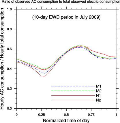
Figure 4. Ratio of AC consumption to total electric consumption averaged for the 10-day EWD period in July 2009 computed with the four methodologies: M1, M2, N1, and N2.
Download figure:
Standard image High-resolution imageThe simulated daily-averaged AC consumption of 185 393.2 MWh (1 MWh = 3.6 × 10⁹ J) is about 1.5 times greater than derived AC consumption for Phoenix (which is calculated from observed SRP data: 58 404.8 MWh × 2.08), with each of the methods outlined previously. The simulated diurnally averaged AC consumption for the entire metropolitan area illustrates the aforementioned overestimate compared to the calculated consumption based on observed utility data (figure 5). It is instructive to examine the source of this bias to provide research guidance on this topic. In present-day BEP + BEM scheme, all urban spaces undergo air conditioning, in contrast to actual environs that realistically do not experience any cooling (e.g., parking structures, home garages). Kikegawa et al (2003), and others more recently (Ohashi et al 2007, Izquierdo et al 2011), estimate the ratio of possible air-conditioned floor area to total floor area as 60%. The cooled relative to the total floor area producing the best correspondence to calculated AC consumption for Phoenix is 65% (figure 5), somewhat higher than the 60% assumed for the cities of Tokyo and Madrid (Kikegawa et al 2003, Ohashi et al 2007, Izquierdo et al 2011). We note that the value of cooled relative to total floor area (65%) is based on the ratio between observed Phoenix AC consumption (obtained using the aforementioned methodologies) and simulated AC consumption.
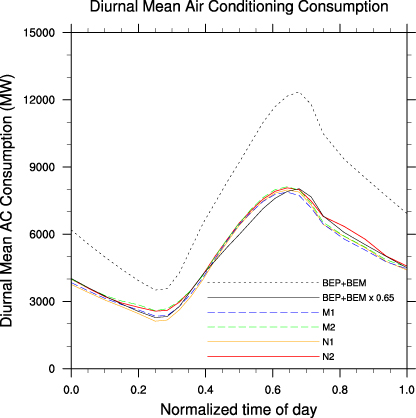
Figure 5. Diurnal mean AC consumption values obtained with the urban scheme and with the four methodologies to estimate the human behavior consumption during the 10-day EWD period in July 2009 (the AC consumption values derived from SRP's data set were multiplied by a factor of 2.08).
Download figure:
Standard image High-resolution imageThe diurnal evolution of observed and simulated AC consumption, as a fraction of total AC consumption for the July 2009 10-day EWD period, are presented as non-dimensional profiles in figure 6(a). The WRF-simulated diurnal pattern of AC consumption strongly resembles each of the four methods, with minimum values apparent shortly after sunrise and peak loads evident prior to sunset.

Figure 6. (a) Non-dimensional AC consumption profiles for the 10-day EWD period in July 2009 computed with the urban module (black line) and with the four methodologies: M1, M2, N1, and N2. (b) Non-dimensional AC consumption profiles obtained with the urban scheme for all the periods studied.
Download figure:
Standard image High-resolution image
The general shape and diurnal evolution of model-simulated and calculated AC consumption (based on observed loads) was apparent for each of the EHEs, with minimal variability among the extreme events exemplified by a small change in amplitude (figure 6(b)). The universality of diurnally averaged non-dimensional AC consumption profiles presented here for EHEs is similar to the universality of total electricity load profiles noted by Sailor and Lu (2004) across diverse geographical areas.
4. Conclusions
In this work, a new methodology to separate the two principal components of the electric consumption has been presented. Hourly load values (supplied by an electric utility company) were split in two parts, one linked to meteorology (AC consumption), and a second linked to human behavior. Based on this principle, four different ways (two methods applied to two different months) to obtain human behavior consumption were developed. Universal non-dimensional AC consumption profiles calculated from observed utility company data were well reproduced, with both the timing and amplitude of maximum and minimum demand correctly simulated with WRF coupled to a multilayer building energy scheme. Electric consumption peaked during evening hours (∼3 pm to ∼6 pm) and the AC demand represented up to ∼65% of the total hourly demand. Assuming 65% of indoor volume is cooled for the Phoenix metropolitan area, a reasonable assumption based on similar cooling volume estimates utilized for the cities of Tokyo and Madrid, the simulation results presented here are in excellent agreement with observationally derived AC consumption data.
This work presents for the first time, to our knowledge, comparison between diurnally averaged model-simulated and observationally derived AC consumption for a number of extreme heat events in a rapidly urbanizing semiarid metropolitan area. The presented methodology, which separates human from meteorological electric consumption, can be applied to assess energy requirements of other rapidly growing metropolitan areas, intended to inform and assist in the future planning of sustainable energy needs of a rapidly urbanizing planet.
Acknowledgments
We gratefully acknowledge the Salt River Project's Forecasting, Research and Economic department for providing electric consumption hourly loads and especially James Walter of the Water Resource Operations department for assistance with the data. We also thank the reviewers for their valuable comments, which led to improvements in this article. This work has been funded by National Science Foundation grants ATM-0934592, DMS-0940314 and the Center for Integrated Solutions to Climate Challenges at Arizona State University.