
Abstract
The production of biofuel from cellulosic residues can have both environmental and financial benefits. A particular benefit is that it can alleviate competition for land conventionally used for food and feed production. In this research, we investigate greenhouse gas (GHG) emissions associated with the production of ethanol, biomethane, limonene and digestate from citrus waste, a byproduct of the citrus processing industry. The study represents the first life cycle-based evaluations of citrus waste biorefineries. Two biorefinery configurations are studied—a large biorefinery that converts citrus waste into ethanol, biomethane, limonene and digestate, and a small biorefinery that converts citrus waste into biomethane, limonene and digestate. Ethanol is assumed to be used as E85, displacing gasoline as a light-duty vehicle fuel; biomethane displaces natural gas for electricity generation, limonene displaces acetone in solvents, and digestate from the anaerobic digestion process displaces synthetic fertilizer. System expansion and two allocation methods (energy, market value) are considered to determine emissions of co-products. Considerable GHG reductions would be achieved by producing and utilizing the citrus waste-based products in place of the petroleum-based or other non-renewable products. For the large biorefinery, ethanol used as E85 in light-duty vehicles results in a 134% reduction in GHG emissions compared to gasoline-fueled vehicles when applying a system expansion approach. For the small biorefinery, when electricity is generated from biomethane rather than natural gas, GHG emissions are reduced by 77% when applying system expansion. The life cycle GHG emissions vary substantially depending upon biomethane leakage rate, feedstock GHG emissions and the method to determine emissions assigned to co-products. Among the process design parameters, the biomethane leakage rate is critical, and the ethanol produced in the large biorefinery would not meet EISA's requirements for cellulosic biofuel if the leakage rate is higher than 9.7%. For the small biorefinery, there are no GHG emission benefits in the production of biomethane if the leakage rate is higher than 11.5%. Compared to system expansion, the use of energy and market value allocation methods generally results in higher estimates of GHG emissions for the primary biorefinery products (i.e., smaller reductions in emissions compared to reference systems).
Export citation and abstract BibTeX RIS

Content from this work may be used under the terms of the Creative Commons Attribution 3.0 licence. Any further distribution of this work must maintain attribution to the author(s) and the title of the work, journal citation and DOI.
1. Introduction
Efforts toward the commercialization of second generation biofuel production have increased in recent years. The production of biofuel from lignocellulosic biomass can improve the sustainability of feedstock production without directly competing with food production. In particular, production of biofuel from cellulosic residues and waste products can alleviate competition for land resources, while reducing the environmental hazards associated with wastes and creating revenue sources for industries that would otherwise pay for waste disposal. Furthermore, the resulting biofuels can displace fossil fuels, reducing greenhouse gas (GHG) emissions.
One of the cellulosic waste materials that can be considered a source for biofuel production is citrus waste (CW). Annual global production of citrus fruits exceeds 88 million tonnes (Marin et al 2007). The majority of this production (70%) is used in the juice and marmalade industries (Marin et al 2007), where about half of the processed citrus, including peels, segment membranes, and seeds ends up as citrus waste (Wilkins et al 2007a). While a portion of CW is dried and used as animal feed, this is typically not economically viable and a large fraction of CW is sent to waste disposal facilities or dumped into the ocean (Yoo et al 2010). New strategies for processing citrus wastes are required to address high disposal costs, a lack of disposal sites, and concerns related to negative environmental impacts from the high organic content of CW and its fermentability (Tripodo et al 2004).
Citrus waste contains carbohydrates that could be hydrolyzed to sugars and used as feedstock for biofuel production. Considering the carbohydrate content of CW (70% of total solid content), there is worldwide ethanol production potential of 1.2 billion liters of ethanol (300 million gallons) from CW (Pourbafrani et al 2010). A novel process for utilizing CW to produce bioethanol, biomethane and limonene has been developed recently at a pilot scale (Pourbafrani et al 2010). This process breaks down carbohydrate polymers to sugar through acid hydrolysis, and then removes inhibitor compounds (limonene) from hydrolyzate. The hydrolyzate's fermentable sugars are converted to ethanol while non-fermentable sugars and other solid residues are digested to produce biomethane. The produced ethanol can be used as fuel, and biomethane can be utilized for electricity generation. The process of conversion of citrus wastes to biofuel was presented in the concept of a biorefinery (Pourbafrani et al 2010) and an analysis of the process shows that the financial feasibility of the process is largely a function of CW cost and supply (Lohrasbi et al 2010). For example, the ethanol production cost is 0.65 USD l−1 at a CW cost of 10 USD/tonne of CW. The cost includes a 0.3 USD l−1 credit for biomethane, based upon a biomethane price of 10 USD/MMBtu and a 0.2 USD l−1 credit for limonene, with limonene priced at 1100 USD/tonne. The ethanol production cost increased to 1.1 USD l−1 at a CW cost of 30 USD/tonne of CW, based upon a 200 000 tonne CW supply (Lohrasbi et al 2010). Due to the currently low CW cost, the fact that enzymes are not required to hydrolyze the CW's carbohydrates into sugar monomers, and the moderate operating conditions in the hydrolysis step, production costs for the CW biorefinery are lower than those associated with other lignocellulosic ethanol processes (Piccolo and Bezzo 2009, Laser et al 2009, Humbird et al 2011). Consequently, as reported by Lohrasbi et al (2010), the process can be financially viable at a relatively low capacity (200 000 tonnes CW yr−1). Utilizing CW generated in Florida (3.5 million tonnes CW yr−1), the biorefinery would produce 137 million liters of ethanol, 147 million cubic meters of biomethane and 31 million liters of limonene. At a smaller scale (e.g., 50 000 tonne CW yr−1), the process is modified resulting in the production of biomethane, limonene and digestate only (i.e., without ethanol), and it can be financially viable under certain conditions (see supplementary information available at stacks.iop.org/ERL/8/015007/mmedia).
Life cycle assessment (LCA) can inform the development and commercialization of emerging biofuel systems by evaluating inputs and discharges associated with all stages of biofuel production. LCA has been used in prior studies of ethanol production from lignocellulosic biomass and its use in light-duty vehicles, typically finding significant reductions in GHG emissions relative to vehicles using gasoline or corn-based ethanol fuels (e.g., Spatari et al 2010, McKechnie et al 2011). Biomethane production from waste sources (e.g., agricultural residues, municipal solid waste) has also been shown to significantly reduce GHG emissions relative to conventional natural gas on a life cycle basis (e.g., Arnold 2011, Adelt et al 2011). However, there have been no prior life cycle studies of biofuel production from CW.
Prior technical and financial feasibility studies of production of biofuel from CW as a feedstock showed promising results (Pourbafrani et al 2010, Lohrasbi et al 2010). These studies did not, however, examine environmental performance of the production of biofuel from CWs. To complement the prior studies, LCA-based studies are necessary to examine the environmental performance of biofuel production from CW. The objective of this study is to quantify life cycle GHG emissions associated with CW biorefinery configurations and to compare the results with those of relevant reference systems. Ethanol, biomethane, limonene and digestate production are examined and various co-product treatment methods are investigated, considering two different biorefinery configurations. The impact of biomethane leakage rate, CW GHG emission and CW transportation distance on the life cycle GHG emissions of products are also studied.
2. Methods
2.1. Life cycle inventory analysis
Life cycle inventory analysis models are developed to quantify GHG emissions from the life cycle stages, including feedstock delivery, biorefinery processes, fuel/product transport, distribution, and bioproduct use (figure 1). A description of LCA methods can be found elsewhere (ISO 14044 2006). 'Best estimate' values of biorefinery design and cradle-to-gate parameters (e.g., from the citrus waste technical studies and existing databases) are utilized in the life cycle inventory models. Alternative co-product treatment methods as well as sensitivity/scenario analyses compliment the 'best estimate' analyses (see sections 2.2–2.6 for details).

Figure 1. Life cycle system boundary for citrus waste biorefineries. Note: in the case of the small biorefinery, ethanol is not produced and its related life cycle stages are omitted. Dashed line indicates life cycle boundary. Cradle-to-gate modules for diesel, gasoline, electricity, sulfuric acid, lime, urea, and phosphate are included within the life cycle boundary.
Download figure:
Standard imageEthanol is assumed to be used as E85 and to displace gasoline in a light-duty vehicle; biomethane is assumed to displace natural gas used for electricity generation (combined cycle facility), and limonene is assumed to displace acetone (Kerton 2009). The digestate from the anaerobic digestion process replaces synthetic fertilizer. Details on substitution ratios for the biorefinery products are detailed in section 2.5. We examine emissions of selected GHGs (CO2, CH4, N2O) reported as CO2 equivalents (CO2eq.) based on 100 yr global warming potentials (IPCC 2006). The functional units are 1 MJ of E85, 1 kWh of generated electricity utilizing biomethane, 1 kg of limonene and 1 kg of digestate.
2.2. Feedstock production, collection and transportation
Currently, CW is considered a waste product of juice production; therefore, emissions associated with crop cultivation and juice production processes are not allocated to the CW in our base analyses (Beccali et al 2009). However, allocation of a portion of these emissions to the CW feedstock is examined in a subsequent sensitivity analysis. For this study, it was assumed that the biorefinery is located in Florida, where 3.5 million tonnes of CW are produced each year. CW is transported to the biorefinery by heavy-duty truck. The distance between the juice factories and the biorefinery is assumed to be 16 km (Zhou et al 2007); a sensitivity analysis is completed on this parameter.
2.3. Citrus waste (CW) to biofuels (ethanol, biomethane), limonene and digestate
Two CW biorefinery designs are considered. The large biorefinery design (hereafter referred to as the large biorefinery) produces ethanol, biomethane, limonene and digestate, and was determined in Lohrasbi et al (2010) to be financially viable if the CW supply is more than 200 000 tonnes yr−1 (figure 2).
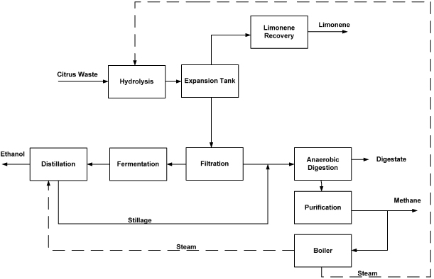
Figure 2. Block flow diagram of large biorefinery (Pourbafrani 2010). Note: the dashed line represents steam, which is generated in the boiler and used in the process.
Download figure:
Standard imageIn the large biorefinery, CW is conveyed to the hydrolysis reactors, where the CW slurry is hydrolyzed using sulfuric acid, with steam injected to the reactors to maintain the temperature at 150 °C. The hydrolyzate is then flashed in an expansion tank to atmospheric pressure, cooling the contents while separating solids and non-volatile components from volatile components that exit as a vapor product stream (Pourbafrani et al 2010). The vapor leaving the expansion tank is condensed and limonene is recovered in a decanter. The solid residue from the hydrolyzate slurry is filtered or centrifuged. The supernatant hydrolyzate is then neutralized and fed to the fermenter (Lohrasbi et al 2010), while the solids are sent to an anaerobic digester. The fermenter 'beer' is fed to distillation columns where ethanol is purified. The stillage from the bottoms of the distillation column is mixed with washed solid residues from the filter/centrifuge, and fed to the anaerobic digestion plant. The anaerobic digester effluent is introduced to the wastewater treatment section of the facility. The sludge, including suspended solids and cell mass, is first settled and removed by gravity sedimentation and filtration. The supernatant effluent is then treated in a conventional wastewater treatment process. The fugitive biomethane emissions are assumed to be 3.1% of the biomethane production rate at normal operation (Flech et al 2011). The steam requirement in the distillation and hydrolysis stages is provided by combusting 29% of the biomethane produced. The product yields of the biorefinery, electricity, process chemical inputs and related GHG emissions are summarized in table 1.
Table 1. Product yields, chemical inputs and electricity used in the citrus waste biorefineries.
| Large biorefinery | Small biorefinery | |
|---|---|---|
| Product yields (/tonne of CW) | ||
| Ethanol (l) | 39.5 | 0 |
| Limonene (l) | 8.9 | 8.4 |
| Biomethane (m3) | 54.3 | 104.7 |
| Digestate (kg) | 44.0 | 41.0 |
| Chemical inputs (kg/tonne of CW) (Lohrasbi 2008) | ||
| Sulfuric acid | 3.8 | 0 |
| Urea | 0.06 | 0 |
| Lime | 5.2 | 0 |
| Phosphate | 0.02 | 0 |
| Electricity use (kWh/tonne of CW)a | 42.0 | 48.0 |
| GHG emissions (kg CO2eq./tonne of CW) | ||
| Transportation of CW | 2.0 | 2.0 |
| Electricity consumption in process | 31.0 | 35.5 |
| Chemicals | 23.7 | 0 |
| Biomethane leakage | 23.2 | 45.8 |
| Total emissions from well to exit gate of biorefinery | ||
| 79.9 | 83.3 | |
| Key LCA assumptions. | ||
| 1—The distance between biorefinery and juice factory is 16 km. | ||
| 2—Heavy-duty trucks are used to transport CW. | ||
| 3—Electricity is imported to biorefineries from Florida's grid. | ||
| 4—LCA boundary includes transportation of CWs, biorefinery stages, product transport and product usage. | ||
| 5—Biomethane leakage rate is 3.1%. | ||
aIncludes electricity consumption at all stages of process including hydrolysis, fermentation, distillation, anaerobic digester and wastewater treatment plant.
The small biorefinery design (hereafter referred to as the small biorefinery), which produces biomethane, limonene and digestate, was determined in Forgacs et al (2011) to be financially viable at a lower CW supply (50 000 tonnes yr−1) (see supplementary information available at stacks.iop.org/ERL/8/015007/mmedia). In the small biorefinery, the carbohydrates in the CW are not hydrolyzed to monomers, and thus, no acid or other chemicals are added (Forgacs et al 2011). The CW slurry is heated and flashed to recover limonene, with the solids and carbohydrate-rich residues sent directly to a biogas digester (figure 3). The ethanol production steps are also omitted. The steam required for heating the CW is provided by combusting 22% of the biomethane produced. The product yields are summarized in table 1.
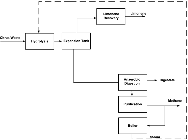
Figure 3. Block flow diagram of small biorefinery (Pourbafrani 2010). Note: the dashed line represents steam, which is generated in the boiler and used in the process.
Download figure:
Standard imageData reported by Lohrasbi et al (2010) and Lohrasbi (2008) for electricity consumption at the CW biorefinery process stages including; hydrolysis, fermentation, anaerobic digestion and waste water treatment plant and chemicals used in the process were utilized in the life cycle model (see table 1). Cradle-to-gate modules for process energy and chemical inputs to the biorefineries are included in the life cycle models. Electricity requirements of the biorefineries are assumed to be supplied by the Florida average electricity generation mix (table 2) (EIA 2011a). The GHG emissions related to purchased electricity are obtained from GREET 1.8C (Argonne National Laboratory 2011). Greenhouse gas emissions associated with the production of process chemicals required during fermentation are obtained from Spatari and MacLean (2010).
2.4. Treatment of biorefinery co-products
Both the large biorefinery and small biorefinery produce multiple products. Prior LCA studies have shown that the treatment of co-products can significantly impact GHG emissions and other metrics associated with the production of the biorefinery products (e.g., Wang et al 2011). In this research, system expansion (displacement) and two allocation methods (market value and energy) are explored in the life cycle modeling of the biorefinery pathways. The International Organization for Standardization suggests that allocation methods (e.g., energy or market value) be used only if allocation cannot be avoided (ISO 14044 2006).
In system expansion, one product is selected as the primary product and all other products are treated as co-products. For the large biorefinery, two displacement scenarios are modeled considering either ethanol or biomethane as the primary product. GHG emissions associated with feedstock transportation and the biorefinery processes are attributed entirely to the primary product, and emissions credits from co-products displacing reference products are assigned to the primary product. The reference products are described in section 2.5. In this work, we focus on the life cycle results using system expansion, but additionally compare these results with those obtained from market value and energy allocation methods, to illustrate differences and highlight key insights.
Allocation of GHG emissions based on market values of the product streams is undertaken considering 2011 market prices of ethanol, biomethane, limonene and digestate: $0.80 USD l−1 (ICIS 2011), $4.5 USD GJ−1 (EIA 2011b), $7.2 USD kg−1 (AAA Chemicals 2012) and $17 USD/tonne (Environment Agency 2010), respectively. Allocation based on energy content is based on the products' higher heating values. This allocation method treats all products as energy products. The higher heating values (HHV) of ethanol, biomethane, limonene and digestate are 21 MJ l−1,36.6 MJ m−3,45 MJ kg−1 and 8 MJ kg−1, respectively. Table 3 summarizes the allocation of biorefinery GHG emissions to products based on their market and heating values. The fractions shown in table 3 were used as allocation factors to attribute biorefinery GHG emissions to products. An interesting observation is that market value versus energy allocation has relatively little influence on allocation of GHG emissions to ethanol, but significantly redistributes the GHG burden between the limonene and methane co-products (table 3).
Table 3. Fraction of inputs and GHG emissions attributed to biorefinery products by co-product treatment method.
| Biorefinery | Co-product method | |||
|---|---|---|---|---|
| System expansion | Market value allocation | Energy allocation | ||
| Large biorefinery | Scenario 1 | Scenario 2 | ||
| Ethanol | 1.00 | (Co-product) | 0.34 | 0.27 |
| Biomethane | (Co-product) | 1.00 | 0.07 | 0.47 |
| Limonene | (Co-product) | (Co-product) | 0.58 | 0.13 |
| Digestate | (Co-product) | (Co-product) | 0.01 | 0.12 |
| Small biorefinery | ||||
| Biomethane | 1.00 | 0.20 | 0.81 | |
| Limonene | (Co-product) | 0.79 | 0.10 | |
| Digestate | (Co-product) | 0.01 | 0.09 | |
2.5. Product transportation, distribution, and use
Ethanol is assumed to be blended with gasoline to produce E85 (83% (v/v) ethanol), which is consumed in a flexible-fuel light-duty vehicle. The E85 and baseline gasoline (35% conventional and 65% reformulated gasoline) vehicles have fuel economies of 10.1 l gasoline equivalent/100 km (Argonne National Laboratory 2011). Biomethane is assumed to displace natural gas in a combined cycle electricity generation facility with an efficiency of 53%. The electricity generation efficiency and associated GHG emissions are obtained from GREET 1.8C (Argonne National Laboratory 2011). Limonene is a biodegradable solvent and can replace products such as acetone in organic solvents (Kerton 2009). The main uses of organic solvents include dissolution of coatings (paints, varnishes, and lacquers), industrial and household cleaners, printing inks and extractive processes. The GHG emissions associated with acetone production from crude oil (2420 gCO2eq. kg−1) were obtained from Wu et al (2008). In this study, we assumed that limonene replaces acetone at the same mass equivalent basis. Digestate is assumed to be utilized as an agricultural fertilizer, displacing synthetic fertilizer, assuming that 50% of its nitrogen content and 100% of its phosphate and potassium could be recovered for this use (Arnold 2011). The NPK (nitrogen, phosphate and potassium) contents of digestate are 120, 26 and 0.5 kg/tonne, respectively. GREET 1.8C (Argonne National Laboratory 2011) includes the GHG emissions related to NPK contents of fertilizer. Based on these emission values, a GHG credit was calculated by assuming that the digestate nutrient content could displace equivalent amounts of synthetic NPK. Digestate is transported using heavy-duty trucks. Citrus farms are assumed to be located an average distance of 30 km from biorefineries.
2.6. Sensitivity and scenario analyses
Parameters such as distance between the biorefinery and juice factory, per cent leakage of biomethane and CW GHG emissions are uncertain and their impacts on life cycle emissions of E85 and biomethane are studied through sensitivity and scenario analyses.
3. Results and discussion
Greenhouse gas emissions associated with the CW transportation and biorefinery stages (well-to-biorefinery exit gate) are 79.9 and 83.3 kg CO2eq./tonne of CW in the large biorefinery and small biorefinery, respectively (table 1). The largest sources of GHG emissions are related to the electricity input, biomethane leakage in the digester, and chemicals used in the large biorefinery. The transportation of CWs is a minor contributor to the GHG emissions and this is in part due to the short transportation distance assumed (16 km) (table 1).
3.1. Large biorefinery
3.1.1. Scenario 1: ethanol as primary product.
For the large biorefinery, the life cycle (well-to-wheel) emissions associated with the E85 flexible-fuel vehicle compared with the reference gasoline vehicle under different co-product treatment methods are shown in table 4. Under system expansion, all biorefinery emissions are attributed to ethanol (70.8 g CO2eq. MJ−1 E85). To provide some perspective, the biorefinery GHG emissions associated with ethanol production from CW are compared with a study that examined ethanol production from other lignocellulosic feedstock. Hsu et al (2010) report considerably lower biorefinery emissions for ethanol from wheat straw, switchgrass and corn stover (9.8 g CO2eq. MJ−1 E85). The higher biorefinery emissions assigned to ethanol in the CW biorefinery are in part due to the lower ethanol yield (200 l dry tonne−1 of CW) compared to that from the other agricultural residues (374 l dry tonne−1). However, other differences between our study and that of Hsu et al (2010) contribute to the difference in emissions. For example, we assume that electricity is imported from the grid whereas Hsu et al assume generation of electricity in the biorefinery from the lignin portion of the feedstock. Furthermore, the CW process must account for emissions due to methane leakage from the anaerobic digester, which is not a factor in the study conducted by Hsu et al.
Table 4. Life cycle GHG emissions associated with citrus waste-based E85 and baseline gasoline and their use in light-duty vehicles under different co-product treatments.
| Life cycle stage | GHG emissions (g CO2eq. MJ−1) | |||
|---|---|---|---|---|
| E85 system expansion | E85 market value allocation | E85 energy allocation | Gasoline | |
| Crude oil recovery | 3.0 | |||
| Transport | 1.8 | 1.0 | 0.5 | 2.5 |
| Biorefinery/crude oil refinery | 70.8 | 24.8 | 19.4 | 13.3 |
| Limonene credit | −20.0 | |||
| Biomethane credit | −85.8 | |||
| Digestate credit | −18.3 | |||
| Ethanol/gasoline transport | 1.5 | 1.5 | 1.5 | 0.6 |
| E85a | 5.1 | 5.1 | 5.1 | |
| Vehicle operationb | 12.8 | 12.8 | 12.8 | 75.6 |
| Total | −32.1 | 45.2 | 39.3 | 95.0 |
aNotes: this value represents the life cycle GHG emissions associated with the gasoline portion of E85. E85 contains 17% (v/v) gasoline and 83% (v/v) ethanol. bThis value represents the GHG emissions associated with the combustion of gasoline.
Co-product credits associated with the use of biomethane, limonene, and digestate are credited to ethanol, resulting in a negative value (−32.1 g CO2eq. MJ−1 E85) for life cycle GHG emissions using system expansion and a large reduction (134%) relative to gasoline (table 4). The negative value results from the GHG emissions credits associated with the three co-products (biomethane, limonene and digestate) being greater than the life cycle emissions attributed to ethanol. The credit associated with biomethane is the largest (−85.8 g CO2eq. MJ−1 E85) due to the high quantity of biomethane that is produced and the assumption that it replaces natural gas. Generation of 1 kWh of electricity from natural gas results in emissions of 480 g CO2eq. (table 5) when employing a combined cycle electricity generation with an efficiency of 53%, and this large amount of CO2eq. emissions is considered as a credit to the life cycle of E85. While a lower efficiency of electricity generation would increase absolute emissions, this would apply to both the biomethane and natural gas-fired systems. Consequently, on a relative basis, the reduction in GHG emissions does not depend upon the electricity generation efficiency and therefore, the co-product credit from biomethane displacing natural gas would remain the same.
Table 5. Life cycle GHG emissions associated with electricity generation from biomethane and baseline conventional natural gas under different co-product treatments.
| Life cycle stage | GHG emissions (g CO2eq. kWh−1) | NGa | |||||
|---|---|---|---|---|---|---|---|
| Large biorefinery | Small biorefinery | ||||||
| System expansion | Market value allocation | Energy allocation | System expansion | Market value allocation | Energy allocation | ||
| CW transport | 9.6 | 2.2 | 5.2 | 5.2 | 3.1 | 4.4 | |
| Biorefinery/NG production | 396.1 | 28.0 | 192.6 | 202.8 | 40.4 | 165.3 | 59.8 |
| Electricity generating station | 8.1 | 8.1 | 8.1 | 8.1 | 8.1 | 8.1 | 420.5b |
| Limonene credit | −112.1 | −54.6 | |||||
| Digestate credit | −102.5 | −50.2 | |||||
| Ethanol credit | −423.5 | ||||||
| Total | −224.3 | 38.3 | 205.9 | 111.3 | 51.6 | 177.8 | 480.3 |
aNotes: NG = conventional natural gas. bThe GHG emissions correspond to electricity generation from natural gas in a combined cycle facility with an efficiency of 53%.
The life cycle GHG emissions associated with E85 produced from CW utilizing system expansion (−32.1 g CO2eq. MJ−1 E85) are considerably lower than those reported by Hsu et al (2010) for E85 produced from wheat straw, corn stover and switchgrass (24, 34 and 32 g CO2eq. MJ−1 E85, respectively). While the CW biorefinery-related emissions for ethanol were higher than those of Hsu et al (2010), the lower ethanol yield in the CW biorefinery results in a correspondingly greater output of co-products and co-product GHG credits. Lower life cycle GHG emissions and lower production costs for the CW biorefinery make CW a promising feedstock for ethanol production.
About one third of the biorefinery GHG emissions are allocated to ethanol under the market value allocation due to the relatively high market value of ethanol (table 3). In contrast, under energy allocation, approximately a quarter of the biorefinery GHGs are allocated to ethanol, due to the relative low energy content of ethanol compared with the other products. As a result of the different allocation procedures, the production and use of ethanol as E85 to displace gasoline reduces GHG emissions by 53% when applying market value allocation and 59% when applying energy allocation (table 4). The difference between the market value and energy allocation results is approximately 10%, whereas even greater differences are noted when comparing with results of the system expansion approach.
3.1.2. Scenario 2: biomethane as primary product.
Life cycle emissions associated with the use of biomethane to produce electricity in a combined cycle facility are compared with the use of conventional natural gas in the same facility (table 5). As in the case of ethanol as a primary product (discussed in section 3.1.1), the lowest GHG emissions are achieved when the system expansion approach is applied to biomethane (147% reduction relative to conventional natural gas). This large reduction is due primarily to a high co-product credit associated with replacing gasoline with ethanol. In all co-product treatment options, emissions associated with biorefinery operations represent the largest fraction of GHG emission over the biomethane life cycle. Based upon system expansion, generation of electricity from biomethane appears favorable.
Biomethane has relatively low market value compared to the biorefinery's other products and only 7% of GHG emissions are allocated to biomethane under the market value allocation scenario. In contrast, methane has a high allocation factor based on energy content, with almost half of the biorefinery GHG emissions are allocated to biomethane when considering energy allocation. Electricity generation from biomethane can reduce GHG emissions by 92% and 57% compared to generation from natural gas when applying market value and energy allocation, respectively (table 5). However, market value allocation creates issues, because the emissions (and emissions reduction) would vary with market price. Thus, among these two methods, energy allocation would provide a more consistent, robust assessment of GHG emissions.
3.1.3. Limonene (large biorefinery).
Due to the high market value of limonene compared to other products, more than half of biorefinery GHGs are allocated to limonene under market value allocation (table 3). The GHG emissions associated with limonene production are 6281 and 1224 g CO2eq. kg−1 of limonene considering market value and energy allocation, respectively (table 6). Considering energy allocation, the GHG emissions allocated to limonene production are approximately 50% lower than those associated with acetone production (2420 g CO2eq. kg−1). In contrast, under market value allocation, the GHG emissions associated with limonene are much higher than those associated with acetone production and with this allocation method, it would not be favorable from a GHG perspective to replace acetone with limonene. As discussed in section 2.5, this study assumes that limonene is functionally equivalent to acetone on a mass basis. Differences in the functional equivalence of limonene and acetone would impact the emissions reduction/increase reported here, as would the consideration of other limonene use scenarios.
Table 6. Life cycle GHG emissions associated with limonene production under different co-product treatments.
| Life cycle stage | GHG emissions (g CO2eq. kg−1 limonene) | |||
|---|---|---|---|---|
| Large biorefinery | Small biorefinery | |||
| Market value allocation | Energy allocation | Market value allocation | Energy allocation | |
| CW transport | 37 | 29 | 57 | 24 |
| Biorefinery | 6224 | 1175 | 9038 | 1009 |
| Transport | 20 | 20 | 20 | 20 |
| Total | 6281 | 1224 | 9115 | 1053 |
3.1.4. Digestate (large biorefinery).
The GHG emissions associated with digestate production are 22.5 and 226 g CO2eq. kg−1 of digestate considering market value and energy allocation, respectively. The low amount of GHG emissions allocated to digestate under market value allocation is due to digestate's low market value (table 3). However, potential fluctuations in the value of digestate (tied to the market value of NPK fertilizer) would affect GHG emissions based on market value allocation. As noted above, among these two options, energy allocation lead to more robust and stable estimates of emissions. Transportation of the digestate represents just 3.8 g CO2eq. kg−1 of digestate. The GHG emissions allocated to digestate, under either allocation method, are considerably lower than those associated with synthetic fertilizer production (461 g CO2eq. kg−1) with the same NPK value as the digestate.
3.2. Small biorefinery
3.2.1. Biomethane.
The life cycle GHG emissions of electricity generation from biomethane are 111.3 g CO2eq. kWh−1 (77% lower than natural gas generated electricity), based upon the system expansion approach (table 5). Despite similar production quantities of limonene and digestate per tonne of CW in both biorefineries (table 1), biomethane production in the small biorefinery is almost twice that of the large biorefinery, and consequently, in the small biorefinery, the co-product credits for limonene and digestate are approximately half of the credits reported for the large biorefinery. Furthermore, there is no ethanol co-product credit in the small biorefinery. Biomethane from the small biorefinery thus leads to a smaller reduction in GHG emissions (relative to natural gas) compared to biomethane produced by the large biorefinery (table 5).
For the small biorefinery, using the energy allocation method, the majority of emissions are allocated to biomethane (81%) due to the high quantity of biomethane produced compared to the quantities of limonene and digestate (table 3). Compared to the large biorefinery, this is a much higher GHG allocation to biomethane (on a percentage basis) since there is no ethanol co-product and the biomethane yield per tonne of CW is approximately double that calculated for the small biorefinery case (table 3). In contrast, due to the relatively low price of biomethane compared to limonene, only 20% of biorefinery GHG emissions are allocated to biomethane under the market value allocation. Electricity generation from biomethane reduces GHG emissions by 90% and by 63% relative to conventional natural gas based electricity generation, using market value and energy allocation, respectively (table 5). As noted above, price fluctuations would influence the emissions reduction determined by market value allocation.
3.2.2. Limonene (small biorefinery).
There is a considerable difference between the share of biorefinery GHG emissions allocated to limonene under market value and energy allocation. The GHG emissions allocated to limonene are 9115 and 1053 g CO2eq. kg−1 of limonene, considering market value and energy allocation, respectively (table 6). As no ethanol is produced by the small biorefinery and biomethane currently has a relatively low market value, a greater fraction of the biorefinery's GHGs is allocated to limonene in small biorefinery compared to large biorefinery under market value allocation (table 3). Similar to the large biorefinery, under the market value allocation approach, GHGs allocated to limonene exceed those of acetone production (2420 g CO2eq. kg−1 of acetone). Variations in the relative values for limonene, methane and digestate would alter the allocated emissions under market value allocation; this variability creates problems when attributing emissions to specific products from a multi-product biorefinery.
3.2.3. Digestate (small biorefinery).
The GHG emissions allocated to the digestate are 24 and 187 g CO2eq. kg−1 of digestate considering market value and energy allocation, respectively. Similar to results for the large biorefinery, the GHG emissions associated to digestate are much lower than those for synthetic fertilizer (461 g CO2eq. kg−1). This large difference in GHG emission between digestate and synthetic fertilizer shows that replacing synthetic fertilizers with digestate produced in CW biorefineries is promising in terms of GHG reduction potential.
3.3. Comparative bioenergy performance of the two biorefineries
The bioenergy products (ethanol and biomethane) resulting from the large biorefinery together have an energy content of 2.3 GJ/tonne of citrus waste, compared to 2.9 GJ/tonne of citrus waste for the small biorefinery's product (biomethane). The lower value for the large biorefinery is due to higher steam consumption per tonne of feedstock in the large biorefinery (required for ethanol production), which therefore uses a greater portion of the produced biomethane (as mentioned in section 2.3). Despite the lower bioenergy yield associated with the large biorefinery, it could be the preferred production scheme in many jurisdictions, due to significant interest in substituting gasoline with ethanol.
3.4. Sensitivity and scenario analyses
3.4.1. Attribution of citrus cultivation and citrus processing GHG emissions to CW.
This study assumes that CW is a waste product of juice production, and therefore no GHG emissions associated with juice production or crop cultivation were allocated to the CW (Beccali et al 2009). While representative of current practice, this assumption may not be valid if competing markets for CW exist. In this case, CW may be considered a co-product of juice production and it may be appropriate to allocate a portion of crop cultivation and production emissions to the CW. Beccali et al (2009) reported energy inputs and GHG emissions related to crop cultivation and juice production among product streams (natural juice, concentrated juice and limonene). We adapt the results of Beccali et al (2009) and allocate a portion of the GHG emissions from citrus cultivation and the primary juice extraction stage to CW. According to Beccali et al (2009), 65% of citrus fruits (orange) ended up as CW on a mass basis. Therefore, we assigned from zero up to a maximum of 65% of GHG emissions of citrus cultivation and the primary juice extraction to CW, resulting in a range of GHG emissions from 0 to 55 kg CO2eq./tonne of CW. Figure 4(a) shows the impact of the CW-related GHG emissions upon the life cycle emissions associated with E85 in the large biorefinery, and upon electricity generation from biomethane in the small biorefinery (assuming system expansion). As the emissions attributed to CW increase, the emissions associated with E85 and electricity generation increase. At the high end (55 kg CO2eq./tonne CW), the life cycle GHG emissions associated with E85 and electricity generation from biomethane are 67.7 g CO2eq. MJ−1 and 368 g CO2eq. kWh−1 respectively. The GHG emissions reduction associated with production and use of E85 compared to gasoline (95 g CO2eq. MJ−1) decreases from 134% to 29% when the emissions associated with CW increase from 0 to 55 kg CO2eq./tonne. GHG emissions reductions of 23% are achieved by the generation of electricity from biomethane compared to generation from natural gas (480 g CO2eq. kWh−1).
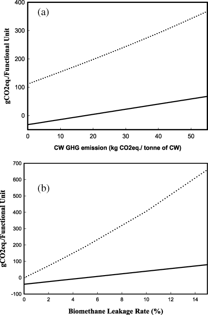
Figure 4. (a) Effect of citrus waste GHG emissions on the life cycle GHG emissions (g CO2eq. MJ−1) of E85 (solid line) in the large biorefinery and on the life cycle GHG emissions (g CO2eq. kWh−1) of electricity generation from biomethane (dashed line) in the small biorefinery, based on system expansion. (b) Effect of biomethane leakage rate (%) on the life cycle GHG emissions (g CO2eq. MJ−1) of E85 (solid line) in the large biorefinery and on the life cycle GHG emissions (g CO2eq. kWh−1) of electricity generation from biomethane (dashed line) in the small biorefinery, based on system expansion.
Download figure:
Standard image3.4.2. Fugitive biomethane emissions.
Another important factor impacting GHG emissions is the fugitive biomethane emissions due to leakage from digesters or the upgrading unit. Previous studies (Arnold 2011, Adelt et al 2011, Flech et al 2011) have shown that fugitive biomethane emissions play an important role in the overall GHG balance of biogas production due to methane's relatively high global warming potential. The amount of fugitive biomethane is uncertain, and can range between 0.1% and 15% of the biomethane production rate, depending on the size of digesters, technology used and operating conditions (Arnold 2011). We utilized system expansion to investigate the effect of fugitive biomethane emissions on the life cycle GHG emissions associated with E85, where the ethanol was produced by the large biorefinery, and with electricity generation from biomethane produced by the small biorefinery (figure 4(b)). At the highest leakage rate (15%), the life cycle GHG emissions associated with E85 and electricity generation are 81.6 g CO2eq. MJ−1 and 606 g CO2eq. kWh−1, respectively. These values are much higher than those associated with E85 (−32.1 g CO2eq. MJ−1) and electricity generation from biomethane (111.3 g CO2eq. kWh−1) at the commonly cited leakage rate of 3.1% (tables 4 and 5). The results show that the leakage of biomethane reduces the difference in GHG emissions between electricity generation from natural gas and biomethane, and if fugitive emissions are high (>11.5%), there will be no GHG emissions benefit resulting from the production of biomethane and its use for electricity generation (figure 4(b)). The leakage of biomethane also increased GHG emissions for E85. If the GHG emissions associated with the E85 are not at least 60% lower than the GHG emissions of gasoline, then the biofuel does not meet the standard for classification as a cellulosic biofuel according to the US Energy Independence and Security Act (EISA 2007). Based on the results presented here, the EISA criterion would not be met if the biomethane leakage rate exceeds 9.7%. At this leakage rate, the life cycle GHG emissions of E85 are 38 g CO2eq. MJ−1. Given the potentially significant impacts of the biomethane leakage on GHG emissions, it is important to carefully design and monitor the process steps (digestion and biomethane purification) where the leakages of biomethane may occur.
3.4.3. CW transportation.
GHG emissions associated with the transportation of CW to the plant depend on the distance between the juice factories and biorefinery. However, each 16 km increase in the distance between the juice factory and biorefinery adds just 0.3 g CO2eq. MJ−1 and 0.7 g CO2eq. kWh−1 to the life cycle GHG emissions of E85 and electricity generation, respectively. Therefore, the transportation distance has a minimal effect on the life cycle GHG emissions of bioproducts, within the range of expected distances.
3.5. Implications of co-product treatment method
The choice of co-product allocation method significantly influences the life cycle GHG emissions of bioethanol. Of the methods examined, the bioethanol produced in the large biorefinery would only meet the EISA requirement for cellulosic ethanol (a 60% reduction of GHG emissions compared to gasoline) when the system expansion approach is applied. When applying the market value and energy allocation methods (table 4), reductions are less than 60% and would not meet EISA's requirement (assuming a biomethane leakage rate of 3.1%).
According to ISO, system expansion is the preferred procedure for attributing emissions to multiple products (ISO 14044 2006) and the procedure is commonly employed in life cycle studies of biofuels. This approach has been used to assess policies aimed specifically at reducing GHG emissions of the transportation sector (e.g., EISA, EPA 2010), although EISA does not prescribe a specific accounting method to address co-products. Economy-wide approaches to regulating GHG emissions may also regulate co-product markets (electricity generation, solvents, fertilizers) and thus may require allocation of GHG emissions across all products. Further, system expansion may not be suitable where co-products represent a significant production output or there is not a definitive primary product (e.g., oil refinery operations). In the present study, either ethanol or biomethane could justifiably be selected as the primary product of the large biorefinery based on product yields.
Allocation approaches, in turn, are limited due to the arbitrary nature of selecting an allocation basis and the lack of consideration of the impact of products displacing alternatives (Weidema 2001). Allocating impacts on the basis of market value is subject to volatility in product prices, which may impact the attributed life cycle GHG emissions. Price variations imply that the GHG emissions reduction could vary from, for example, year to year, or between jurisdictions. In jurisdictions that have a cost on carbon emissions, or in jurisdictions that stipulate GHG reductions as part of their renewable fuel standards, such variations would create regulatory and administrative complications. The main drawback of energy allocation in the case of biorefinery operations is that not all products may be fuels: in the present study, limonene and digestate are treated as energy products during allocation, but are ultimately not used as such. Furthermore, it is difficult to disaggregate process inputs among specific products that are typically produced and purified in the same process unit operations.
4. Conclusion
The life cycle-based examination of the CW biorefineries shows that considerable GHG reductions may be achieved by utilizing the products of the large and small biorefineries. For the large biorefinery, ethanol used as E85 in a light-duty vehicle results in a 134% reduction in GHG emissions compared to a gasoline-fueled vehicle, when utilizing system expansion. For the small biorefinery, GHG emissions are reduced by 77% when electricity is generated from biomethane rather than natural gas, when applying system expansion. Limonene and digestate replace acetone and fertilizer, respectively, and these replacements result in credits to the life cycle GHG emissions of the produced biofuels. The magnitude of the GHG emissions reductions for the biorefinery products is strongly dependent on fugitive emissions of biomethane. Compared to system expansion, market value and energy allocation methods generally resulted in higher GHG emissions being assigned to the biofuel. Overall, CW biorefineries show promise because they can use a 'waste' feedstock to produce multiple products that can displace fossil reference products, while significantly reducing life cycle GHG emissions.
Acknowledgments
We thank the Government of Canada through AUTO21 Network Centre of Excellence, Genome Canada (2009-OGI-ABC-1405), and the Natural Sciences and Engineering Research Council, as well as General Motors and the Government of Ontario (ORF-GL2-01-004) for financial support.