
Abstract
Temporal and spatial patterns in northern midlatitude atmospheric ozone levels measured outside the cabin by MOZAIC aircraft are investigated to consider trends in human exposure to ozone during commercial flights. Average and 1 h peak ozone levels for flights during 2000 to 2005 range from 50 to 500 ppb, and 90 to 900 ppb, respectively, for flights between Munich and New York (N = 318), or Chicago (N = 372), or Los Angeles (N = 175). Ozone levels vary through the year as expected on the basis of known trends in tropopause height. Timing and amplitude of the mean annual cycle are consistent across routes. A linear regression model predicts flight average and 1 h peak levels that are, respectively, 180 ppb and 360 ppb higher in April than during October–November. High ozone outliers to the model occur in January–March in the western North Atlantic region and may be linked to episodic stratosphere-to-troposphere exchanges. No systematic variation in atmospheric ozone is observed with latitude for the routes surveyed. On average, ozone levels increase by 70 ppb per km increase in flight altitude, although the relationship between altitude and ozone level is highly variable. In US domestic airspace, ozone levels greater than 100 ppb are routinely encountered outside the aircraft cabin.
Export citation and abstract BibTeX RIS

Content from this work may be used under the terms of the Creative Commons Attribution-NonCommercial-ShareAlike 3.0 licence. Any further distribution of this work must maintain attribution to the author(s) and the title of the work, journal citation and DOI.
1. Introduction
Ozone is found at high concentrations in the stratosphere where its formation is initiated by the UV-photolysis of oxygen. Commercial passenger airplanes, which routinely fly at cruise altitudes between 9 and 13 km, encounter elevated ozone when they cross the tropopause. Tropopause height varies spatially and seasonally, from a mean value of 15–18 km in the tropics to 6–8 km near the poles, and with a spring minimum and a fall maximum. The change in tropopause height with latitude is neither linear nor constant, but exhibits sharp discontinuities. Most notably, it jumps across the jet stream. Moreover, tropopause height can fluctuate over short periods owing to meteorological processes (NRC 2002, Holton et al 1995) that cause stratosphere-to-troposphere exchange (STE). The STE events are associated with mesoscale fluctuations and are most common (in the northern hemisphere) in the midlatitudes (30–60°N) (Stohl et al 2003, El Amraoui et al 2010). These episodic processes are classified by Stohl et al (2003) into two types, one of which—deep STE—has a strong winter maximum and summer minimum and a distinct geographical pattern, including an association with storm tracks (Holton et al 1995, Morgenstern and Marenco 2000).
Acute health effects attributed to short-term inhalation exposure to ozone and its volatile reaction byproducts range from breathing discomfort, respiratory irritation, and headache for healthy adults (Strøm-Tejsen et al 2008) to asthma-exacerbation and premature mortality for vulnerable populations (Gent et al 2003, Bell et al 2004). Chronic exposure effects may include enhanced oxidative stress (Chen et al 2007), reduced lung function in young adults (Tager et al 2005), and adult-onset asthma in males (McDonnell et al 1999). While ground-level ozone is a regulated pollutant, stratospheric ozone is considered beneficial because of its location away from humans, and its role in protecting the earth from potentially harmful ultraviolet radiation. However, humans can be exposed to stratospheric ozone during air travel. Levels inside the cabin are reduced relative to atmospheric levels encountered by aircraft owing to ozone reactions with cabin interiors on all aircraft and owing to the use of control devices known as 'ozone converters' on some aircraft.
Measurements of ozone made in occupied cabins during flight are the most direct means of assessing in-cabin exposures and consequent health risks. A recent in-cabin ozone survey found that mean and peak 1 h ozone levels were low (less than 10 ppb) on US domestic flights equipped with ozone converters (Bhangar et al 2008). On domestic flights without converters levels were higher, with peak 1 h ozone greater than 100 ppb in 10% of the sample. Another in-cabin ozone survey of airplanes on domestic, Pacific, and southeast Asian routes measured flight average or 3 h mean levels exceeding 100 ppb on 20% of flights sampled, suggesting that the aircraft sampled either lacked converters or that the converters, if present, were not functioning effectively (Spengler et al 2004). Since in-cabin data are expensive and time consuming to acquire and recently acquired data are therefore scarce, the present analysis seeks to elucidate an important factor influencing ozone exposures in aircraft: atmospheric ozone levels along commercial passenger flight routes.
Since 1994, the MOZAIC (measurement of ozone and water vapor by Airbus in-service aircraft) campaign has measured ozone levels along numerous flight routes, with a bias toward the North Atlantic corridor (Marenco et al 1998). Previous research utilizing MOZAIC ozone data has evaluated the effects of airplanes on atmospheric composition; identified and explained spatial and temporal ozone trends in the upper troposphere and lower stratosphere (UT/LS) region; assessed the frequency and features of cross-tropopause ozone flows; and evaluated three-dimensional chemistry and transport models (MOZAIC 2012). Data from a previous aircraft-based sampling campaign (the Global Atmospheric Sampling Program, GASP) were used to better understand in-cabin ozone trends in the 1970s (Perkins et al 1979). However, the MOZAIC data have not yet been analyzed with a per-flight perspective to consider implications for human exposure to ozone in aircraft cabins during flight.
The present study analyzes time-resolved ozone data collected by MOZAIC flights undertaken in 2000–5, focusing on flight routes between Munich and three major cities that span the continental United States. The study objectives are to assess the distribution of ozone levels encountered by commercial passenger flights on transatlantic routes, to evaluate the influence of season, latitude and altitude on these levels, and to consider implications for exposures within aircraft cabins.
2. Methods
The MOZAIC campaign involves the automatic, regular measurement of various airborne species and variables by five passenger aircraft (Airbus Model A340) during routine commercial flight, utilizing sensors installed on the aircraft shell. Data are collected at irregular intervals, at the approximate frequency of 0.25 Hz. Ozone was measured via dual beam ultraviolet absorption (detection limit 2 ppb; precision ± [2 ppb + 2%]) (Law et al 1998). Flights are monitored at the approximate frequency of 2000 segments per year (Marenco et al 1998). A segment is defined as one nonstop flight between two airports. The aircraft fly at cruising altitudes that range from approximately 9.8 to 12.5 km (Marenco et al 1998).
The present analysis considers all MOZAIC flights between Munich and New York (NY), Chicago, and Los Angeles (LA), during the six-year period between 2000 and 2005. The period from 2000 to 2005 is believed to be reasonably representative of current conditions. Munich was chosen as it is one of the three European cities most frequented by MOZAIC flights. New York, Chicago and LA were selected because they are major cities in the eastern, central, and western US. Flights to these cities comprise 51% of all MOZAIC flights involving a US city (and 18% of the global dataset) during the selected period. Finally, the three cities had approximately even sample sizes (NY =361; LA =274; Chicago =432), and were monitored during all months of the year. Flight segments with more than 10% of data missing were excluded from the analysis. This criterion reduced the numbers of analyzed segments to NY =318, LA =175, and Chicago = 372.
3. Results and discussion
3.1. Comparing means
Sample flight tracks and average flight latitudes corresponding to each route are shown in figure 1. Figure 2 presents cumulative distributions of peak 1 h and flight-average ozone levels obtained from the 865 analyzed flight segments, stratified by route. The data conform reasonably to lognormal distributions. Across all 865 flights, ozone levels span an order of magnitude, with 1 h peak and flight-average ozone ranging from approximately 90 to 900 ppb, and 50 to 500 ppb, respectively. Peak 1 h and flight-average-weighted geometric means are in the ranges 355–415 ppb and 148–209 ppb, respectively. Weighting was done to minimize bias, as data from previous monitoring studies show that ozone levels vary markedly through the year. Variations in ozone levels within each route are substantially greater than the variation across routes.
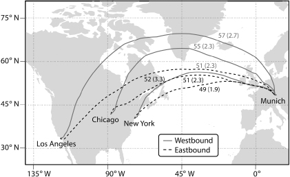
Figure 1. Sample flight tracks for the routes between Munich and each of three US cities. The tracks shown correspond to flights selected at random from a period also selected at random: June–July 2005. The numbers near each trace are the average (standard deviation) flight latitudes for all flights on that route. For all routes, westbound travel traces higher latitudes compared to eastbound travel, and flights with a greater east–west span fly at higher latitudes.
Download figure:
Standard image
Figure 2. Weighted cumulative distributions of peak 1 h (upper trace) and sample-average (lower trace) ozone mixing ratios sampled outside passenger cabins of aircraft on six transatlantic routes. All flights either originated from or terminated in Munich. The weighted geometric mean and standard deviation and lognormal fits using these parameters are presented for each distribution. Data apply for the years 2000–2005.
Download figure:
Standard image3.2. Temporal variability
Figure 3 presents peak 1 h ozone mixing ratios from the 865 flight segments, plotted against time of year. On all six routes, ozone varies through the year in a cyclical manner, and the timing and amplitude of the cycle is similar across routes. The size and statistical significance of the seasonal effect and of the effect of route direction (eastbound or westbound) and US arrival or departure city (LA, NY, or Chicago) were determined by modeling the annual trend using the regression model shown in (1):


Figure 3. Peak 1 h atmospheric ozone encountered by aircraft on westbound (WB) and eastbound (EB) flights between Munich and each of three US cities (N = 865), plotted against time of year. Least-squares best-fit sinusoidal curves (1) are fit to data corresponding to each route.
Download figure:
Standard imageHere the response variable (Y) is the peak 1 h ozone and β0 is the annual mean. The continuous variable x1 is the date, converted to a real number between 0.003 (1 January) and 1.0 (31 December). The magnitude of the seasonal effect is indicated by the relative size of 2β1 in relation to β0. The times at which the maximum and minimum are attained are reflected in the value of ϕ. The effect of the route on the annual mean is encompassed in the last three terms. For westbound routes, WB = 1; for eastbound routes, WB = 0. Similarly, LA = 1 for flights to or from Los Angeles, and NY = 1 for flights to or from New York.
Sinusoidal curves described by the model (r2 = 0.98) are shown in figure 3. Least-squares best-fit values of model parameters are summarized in table 1. Results show that the seasonal effect is large and statistically significant, with peak 1 h levels expected to be 360 ppb higher in April than in October–November. Table 1 also summarizes parameter values obtained by fitting (1) to flight-average ozone levels. The seasonal cycle is consistent across the two metrics—peak 1 h and flight-average ozone—in terms of the timing of the annual high and annual low (ϕ = 6.0–6.1 rad). The predicted annual mean, and the amplitude of the seasonal cycle, are half as large for flight-average ozone levels compared to peak 1 h ozone levels.
Table 1. Summary of least-squares best-fit parameters for the model in (1).
| Effect | Parameter | Peak 1-h ozone | Time-weighted-average ozone | ||
|---|---|---|---|---|---|
| Size | SE | Size | SE | ||
| Annual mean | β0 | 416 ppb | 5.1 ppb | 203 ppb | 3.2 ppb |
| Season (amplitude) | β1 | 182 ppb | 3.9 ppb | 92 ppb | 2.5 ppb |
| Season (phase shift) | ϕ | 6.0 rad | 0.024 rad | 6.1 rad | 0.029 rad |
| Westbound–Eastbound | β2 | 29 ppb | 5.6 ppb | 28 ppb | 3.6 ppb |
| LA–Chicago | β3 | −38 ppb | 7.6 ppb | −40 ppb | 4.8 ppb |
| NY–Chicago | β4 | −21 ppb | 10.9 ppb | −19 ppb | 6.9 ppb |
The finding of higher ozone in April and lower ozone in October–November was expected based on known annual changes in the representative mean height of the tropopause; flights at normal cruising altitudes have a higher chance of crossing into the lower stratosphere and encountering elevated ozone in the spring than during autumn. Previous research on in-cabin and flight-corridor ozone substantiates this expectation (Brabets et al 1967, Spengler et al 2004, Bhangar et al 2008). Data reported by NRC (2002) on ozone levels at flight altitude for selected months and latitudes are also consistent with the observed trend in terms of the timing of the annual cycle, and the magnitude of differences between spring and fall.
In addition to the mean seasonal trend—which is captured well by sinusoidal curves and was expected based on previous research—the degree of scatter about the mean trend also varies throughout the year. A plot of model residuals (measured ozone minus modeled ozone) versus time of year for peak 1 h and flight-average ozone (figure 4) shows large positive model outliers clustered in the months of winter and early spring. The time of year when very high ozone levels are most frequent, and the concentration of high ozone peaks in a region around the western North Atlantic (figure S1 available at stacks.iop.org/ERL/8/014006/mmedia), suggest that episodic stratosphere-to-troposphere exchanges may account for the observed outliers.
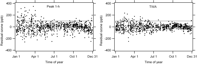
Figure 4. Model residuals (measured ozone minus modeled ozone) versus time of year for peak 1 h and flight-average ozone (N = 865). The dotted line at 100 ppb is intended to guide the eye, and shows that large positive outliers to the model (where measured minus modeled ozone exceeds +100 ppb) occur most frequently around February and March.
Download figure:
Standard imageThe hypothesis that the highest ozone levels encountered by aircraft are linked to episodic, local reductions in tropopause height is supported by observations of in-cabin ozone levels on 68 domestic US flight segments (Bhangar et al 2008). The highest ozone level recorded during the study was measured in February and also constituted a strong outlier to the mean seasonal trend in cabin ozone levels. The flight on which this highest level was measured coincided with a major storm that was linked to a tropopause-folding event, and the associated enhanced vertical mixing was hypothesized as the cause of the high ozone observations. Similarly, Jaffe and Estes (1964) linked unusually high atmospheric and in-cabin ozone levels on a US flight to a severe storm. Van Heusden and Mans (1978) observed that crossings of the representative mean tropopause did not explain an ozone peak on a westbound transatlantic flight.
3.3. Spatial variability
The relationship between flight latitude and atmospheric ozone was visually evaluated by mapping ozone measurements for all flights in June (N = 66, figure S2 available at stacks.iop.org/ERL/8/014006/mmedia) on a latitude/longitude grid, with flight altitude segregated into four ranges. June was chosen to observe mean trends because ozone levels in June are well predicted by the model described by (1). The spatial map showed that, within the range of latitudes sampled, there is no monotonic association between latitude and ozone. Elevated levels are distributed across most regions encompassed by the flight tracks investigated, with a band of low ozone in a region that roughly corresponds to the plains states in the continental US and extending as far as northern Manitoba, Canada. Limited observations from in-cabin ozone investigations are consistent with these spatial patterns. Brabets et al (1967) found a similar pattern of low ozone on flight tracks overlaying the US plains states. Bhangar et al (2008) found no latitude-related trend for in-cabin ozone levels for non-converter flights within the continental US.
The absence of an association between latitude and ozone observed for the northern hemisphere western midlatitudes explains why, as summarized in table 1, one observes higher average ozone levels on flight routes to Chicago and NY as compared to flights to Los Angeles. Based on between-flight differences in latitude alone, ozone levels are expected to increase in proportion to the east–west span of a route (within a hemisphere), because longer flights venture further north to trace great circle routes (figure 1). However, by traversing higher latitudes, flights between Munich and LA avoid much of the 'high ozone' region (figure S1 available at stacks.iop.org/ERL/8/014006/mmedia) that is centered in the western North Atlantic and therefore encounter lower average ozone levels than on flights between Munich and Chicago or Munich and New York.
To investigate a between-flight difference attributable to altitude, the association between model residuals and altitude is evaluated (figure S3 available at stacks.iop.org/ERL/8/014006/mmedia). The two parameters are weakly, but consistently and positively associated (linear regression coefficient of determination r2 = 0.2). The slopes of each fit suggest a mean variation on the scale of 70 ppb ozone per km increase in cruising altitude for both peak 1 h and flight-average ozone. This value is broadly consistent with data on the annual mean vertical distribution of ozone presented by NRC (2002).
To assess the contribution of altitude to differences in ozone levels encountered during each flight, the mean flight altitude is compared with the mean altitude at which the 1 h peak is logged, by route (figure S4 available at stacks.iop.org/ERL/8/014006/mmedia). Flights typically gain altitude with elapsed time until just before descent. Consequently, the fraction of flight time that elapses before the occurrence of the 1 h ozone peak is also evaluated, by route, as a second indicator of the influence of altitude on within-flight ozone levels (table S1 available at stacks.iop.org/ERL/8/014006/mmedia). These analyses show that the 1 h ozone peak for each flight segment is, on average, encountered during the second half of a flight (54–64% of time into the flight) on both eastbound and westbound routes, when the flight altitude is 0.7–1 km greater than the overall mean flight altitude.
The effect of altitude relative to effects of the other spatial coordinates (i.e. latitude/longitude) is further resolved by analyzing the 'location', in terms of flight hours away from Munich, of the 1 h ozone peak per flight (table S2 available at stacks.iop.org/ERL/8/014006/mmedia). For flights to Munich, the 1 h ozone peak was encountered 3.2–3.9 h flight time from Munich. For flights from Munich, the 1 h ozone peak was encountered 4.9–6.4 h from Munich, with the distance from Munich scaling in relation to the duration of the flight. The flight times and distances discussed are evidence of the combined influence of two spatial trends in ozone levels encountered by aircraft. First, flights encounter peak levels of ozone in the latitude/longitude zone that corresponds to the 3–7 h 'distance' from Munich. As mean flight speed is approximately 850 km h−1, this travel time corresponds to about 2500–6000 km away from Munich along flight tracks (sample flight tracks are shown in figure 1) in a spatial zone centered in the western North Atlantic. Second, within the latitude and longitude zone of high atmospheric ozone levels, differences in the location of the peak are sensitive to differences in flight altitude.
3.4. Implications for in-cabin ozone exposures
The present investigation reinforces the expectation that aircraft flying on northern midlatitude routes routinely encounter high ozone levels. Without a control device (a catalyst or 'converter') to remove ozone from the ventilation air before it enters the cabin, corresponding in-cabin levels of ozone and ozone reaction byproducts could be unacceptably high—especially between January and June—commonly exceeding limits of 0.1 ppm (3 h average, sea-level equivalent) and 0.25 ppm specified in US Federal Aviation Regulations (FAR 25.832 and FAR 121.578).
A parameter known as the 'retention ratio' (or R-value) is defined as the within-cabin proportion of outdoor ozone in the absence of a control device. The R-value depends on parameters such as cabin surface materials, occupant density, the surface area to volume ratio, and the design and operation of the aircraft ventilation system. R-values between 0.47 and 0.83 were obtained in studies where cabin and ambient ozone levels were measured simultaneously on commercial passenger aircraft (Boeing 747, DC-10) without ozone removal systems (Van Heusden and Mans 1978, Nastrom et al 1980). R-values in the range 0.2–0.4 were inferred by Coleman et al (2008), based on chamber experiments measuring ozone consumption on materials found in aircraft cabins, combined with a common range of cabin air exchange rates and expected in-cabin airflow conditions. For demonstrating compliance with FAA ozone regulations, aircraft can be assigned a default R-value of 0.7 (NRC 2002).
Assuming R = 0.7 and also that ozone converters are absent or ineffective, flight-average ozone levels would exceed 100 ppb on more than 95% of the flights analyzed in this study for the period between February and June. Such high ozone levels would be expected to be accompanied by correspondingly high levels of ozone reaction byproducts (Weschler et al 2007). Based on experiments in an occupied simulated cabin, the total byproduct yield is predicted to range from 0.25 to 0.30 mol of volatile byproduct per mole of ozone consumed (Weschler et al 2007). Owing to reactions occurring on the body envelope, levels of byproducts in the passenger breathing zone are expected to be even greater than average levels in the cabin (Wisthaler and Weschler 2010, Nazaroff and Weschler 2010).
As flights on transatlantic routes are routinely equipped with ozone converters (in response to the introduction of the FARs limiting cabin ozone), this illustrative discussion serves both to demonstrate the exposures avoided through use of effective converters, and to define worst-case scenarios for conditions where a converter is absent or fails to perform adequately. Next, we consider in-cabin levels of ozone that might be expected on the current fleet of aircraft plying transatlantic routes. When new, converters on these aircraft have an expected ozone destruction efficiency (η) of 90%–98% (NRC 2002). If the aircraft in our sample are modeled as having a converter with η = 0.95, and R = 0.7, ozone levels in the cabin are effectively controlled, with predicted in-cabin flight-average and 1 h peak ozone levels less than 18 ppb and 33 ppb, respectively, across all 865 flights investigated.
However, the efficiency of the catalysts tends to degrade with use, and they are subject to replacement or maintenance once the efficiency drops below approximately 60% (Heck et al 1992). At η = 60%, results indicate that in-cabin ozone exposures could be substantial on transatlantic routes. For example, with η = 0.60 and R = 0.7, 97% of flights in the months February–June (and 55% of all flights) would have predicted in-cabin peak 1 h ozone levels exceeding 100 ppb; 6% of all flights would have in-cabin flight-average ozone levels exceeding 100 ppb. These observations highlight the importance not only of equipping transatlantic flights with converters, but also ensuring that they function well throughout their service life.
Maps of the spatial distribution of ozone along the flight routes investigated show that even on domestic US routes (which are frequently traversed by aircraft without ozone converters), elevated ozone levels of hundreds of ppb are routinely encountered in the winter and spring months. Therefore the present investigation supports the benefit of using ozone converters to reduce ozone exposure in all airplanes capable of transcontinental flight.
Flight-route planning is one method that airlines can use to comply with ozone FARs. Data to aid with planning efforts are based on statistical summaries of atmospheric ozone as a function of altitude, latitude, and month (NRC 2002). The results presented here indicate that planning-based risk management techniques may be effective in predicting ozone trends based on month and altitude. However, in addition to being based on mean trends in the position of the tropopause, planning should take account of the intermittent influence of stratosphere-to-troposphere exchange events, especially when considering ozone that might be encountered in the winter months. Moreover, our results suggest that within the transatlantic flight corridor, latitude is not associated monotonically with ozone, so flight-route planning based on expected latitude trends may not be effective.
Acknowledgments
The authors gratefully thank Beverly Coleman and Charles Weschler for providing early feedback and guidance. We acknowledge for their strong support the European Commission, Airbus, and the airlines (Lufthansa, Air France, Austrian and former Sabena) who have carried, free of charge, the MOZAIC instrumentation and performed necessary maintenance since 1994. MOZAIC is presently funded by INSU-CNRS (France), Météo-France, and Forschungszentrum (FZJ, Julich, Germany). The MOZAIC database is supported by ETHER (CNES and INSU-CNRS). The work reported in this paper was funded by the US Federal Aviation Administration (FAA) Office of Aerospace Medicine through the Air Transportation Center of Excellence for Airliner Cabin Environment Research (ACER), Cooperative Agreement 04-C-ACE-UCB. Although the FAA has sponsored this project, it neither endorses nor rejects the findings of this research.