
Abstract
Globally, bioethanol is the largest volume biofuel used in the transportation sector, with corn-based ethanol production occurring mostly in the US and sugarcane-based ethanol production occurring mostly in Brazil. Advances in technology and the resulting improved productivity in corn and sugarcane farming and ethanol conversion, together with biofuel policies, have contributed to the significant expansion of ethanol production in the past 20 years. These improvements have increased the energy and greenhouse gas (GHG) benefits of using bioethanol as opposed to using petroleum gasoline. This article presents results from our most recently updated simulations of energy use and GHG emissions that result from using bioethanol made from several feedstocks. The results were generated with the GREET (Greenhouse gases, Regulated Emissions, and Energy use in Transportation) model. In particular, based on a consistent and systematic model platform, we estimate life-cycle energy consumption and GHG emissions from using ethanol produced from five feedstocks: corn, sugarcane, corn stover, switchgrass and miscanthus.
We quantitatively address the impacts of a few critical factors that affect life-cycle GHG emissions from bioethanol. Even when the highly debated land use change GHG emissions are included, changing from corn to sugarcane and then to cellulosic biomass helps to significantly increase the reductions in energy use and GHG emissions from using bioethanol. Relative to petroleum gasoline, ethanol from corn, sugarcane, corn stover, switchgrass and miscanthus can reduce life-cycle GHG emissions by 19–48%, 40–62%, 90–103%, 77–97% and 101–115%, respectively. Similar trends have been found with regard to fossil energy benefits for the five bioethanol pathways.
Export citation and abstract BibTeX RIS

Content from this work may be used under the terms of the Creative Commons Attribution 3.0 licence. Any further distribution of this work must maintain attribution to the author(s) and the title of the work, journal citation and DOI.
1. Introduction
Globally, biofuels are being promoted for reducing greenhouse gas (GHG) emissions, enhancing the domestic energy security of individual countries and promoting rural economic development. In a carbon-constrained world, liquid transportation fuels from renewable carbon sources can play an important role in reducing GHG emissions from the transportation sector (IEA 2012). At present, the two major biofuels produced worldwide are (1) ethanol from fermentation of sugars primarily in corn starch and sugarcane and (2) biodiesel from transesterification of vegetable oils, with ethanol accounting for the majority of current biofuel production. Figure 1 shows the growth of annual ethanol production between 1981 and 2011 in the US and Brazil, the two dominant ethanol-producing countries.
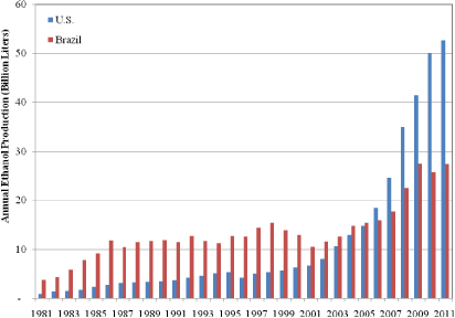
Figure 1. Annual ethanol production in the US and Brazil (based on data from the Renewable Fuels Association (RFA 2012) and Brazilian Sugarcane Association (UNICA 2012)).
Download figure:
Standard imageThe production of corn ethanol in the US has increased to more than 52 billion liters since the beginning of the US ethanol program in 1980. The increase after 2007, the year the Energy Independence and Security Act (EISA) came into effect, is remarkable. Growth in the production of Brazilian sugarcane ethanol began in the 1970s when the Brazilian government began to promote its production. The most recent growth in sugarcane ethanol production, since 2001, has mainly resulted from the popularity of ethanol flexible-fuel vehicles and from the advantageous price of ethanol over gasoline in Brazil.
Over the long term, the greatest potential for bioethanol production lies in the use of cellulosic feedstocks, which include crop residues (e.g., corn stover, wheat straw, rice straw and sugarcane straw), dedicated energy crops (e.g., switchgrass, miscanthus, mixed prairie grasses and short-rotation trees) and forest residues. The resource potential of these cellulosic feedstocks can support a huge amount of biofuel production. For example, in the US, nearly one billion tonnes of these resources are potentially available each year to produce more than 340 billion liters of ethanol per year (DOE 2011). This volume is significant, even when compared to the annual US consumption of gasoline, at 760 billion ethanol-equivalent liters (EIA 2012).
The GHG emission reduction potential of bioethanol, especially cellulosic ethanol, is recognized in policies that address reducing the transportation sector's GHG emissions (i.e., California's low-carbon fuel standard (LCFS; CARB 2009), the US renewable fuels standard (RFS; EPA 2010) and the European Union's renewable energy directive (RED; Neeft et al 2012)). Nonetheless, the life-cycle GHG emissions of bioethanol, especially those of corn-based ethanol, have been subject to debate (Farrell et al 2006, Fargione et al 2008, Searchinger et al 2008, Liska et al 2009, Wang et al 2011a, Khatiwada et al 2012). With regard to corn ethanol, some authors concluded that its life-cycle GHG emissions are greater than those from gasoline (Searchinger et al 2008, Hill et al 2009). Others concluded that corn ethanol offers reductions in life-cycle GHG emissions when compared with gasoline (Liska et al 2009, Wang et al 2011a). On the other hand, most analyses of cellulosic ethanol reported significant reductions in life-cycle GHG emissions when compared with those from baseline gasoline. Reductions of 63% to 118% have been reported (Borrion et al 2012, MacLean and Spatari 2009, Monti et al 2012, Mu et al 2010, Scown et al 2012, Wang et al 2011a, Whitaker et al 2010). Most of these studies included a credit for the displacement of grid electricity with electricity co-produced at cellulosic ethanol plants from the combustion of lignin. Some, however, excluded co-products (e.g., MacLean and Spatari 2009). Uniquely, Scown et al (2012) considered land use change (LUC) GHG emissions (for miscanthus ethanol) and estimated total net GHG sequestration of up to 26 g of CO2 equivalent (CO2e)/MJ of ethanol. In the case of sugarcane ethanol, Seabra et al (2011) and Macedo et al (2008) reported life-cycle GHG emissions that were between 77% and 82% less than those of baseline gasoline. Wang et al (2008) estimated this reduction to be 78%.
A detailed assessment of the completed studies requires that they be harmonized with regard to the system boundary, co-product allocation methodology, and other choices and assumptions that were made. Other researchers (e.g., Chum et al 2011) have undertaken this task to some extent. Here we instead use a consistent modeling platform to examine the GHG impacts from using corn ethanol, sugarcane ethanol and cellulosic ethanol. The GREET (Greenhouse gases, Regulated Emissions, and Energy use in Transportation) model that we developed at Argonne National Laboratory has been used by us and many other researchers to examine GHG emissions from vehicle technologies and transportation fuels on a consistent basis (Argonne National Laboratory 2012). The GREET model covers bioethanol production pathways extensively; we have updated key parameters in these pathways based on recent research. This article presents key GREET parametric assumptions and life-cycle energy and GHG results for bioethanol pathways contained in the GREET version released in July 2012. Moreover, we quantitatively address the impacts of critical factors that affect GHG emissions from bioethanol.
2. Scope, methodology, and key assumptions
We include bioethanol production from five feedstocks: corn grown in the US, sugarcane grown in Brazil, and corn stover, switchgrass and miscanthus, all grown in the US. Even though the wide spread drought in the US midwest in the summer of 2012 may dampen corn ethanol production in 2012, corn ethanol production will continue to grow, possibly exceeding the goal of 57 billion liters per year in the 2007 EISA. Likewise, Brazil's sugarcane ethanol production will continue to grow. In the US midwest corn belt, up to 363 million tonnes of corn stover can be sustainably harvested in a year (DOE 2011). Large-scale field trials have been in place to collect and transport corn stover (Edgerton et al 2010). Switchgrass is a native North American grass. Field trials of growing switchgrass as an energy crop have been in place since the 1980s. Miscanthus, on the other hand, has a high potential yield per acre. In the past several years, significant efforts have been made in the US to develop better varieties of miscanthus with higher yields (Somerville et al 2010).
We conducted the well-to-wheels (WTW, or, more precisely for bioethanol, field-to-wheels) analyses of the five bioethanol pathways with the GREET model (Argonne National Laboratory 2012, Han et al 2011, Dunn et al 2011, Wang et al 2012). In particular, we used the most recent GREET version (GREET1_2012) for this analysis to conduct simulations for the year 2015. Figure 2 presents the system boundary for the five bioethanol pathways in our analysis. Parametric details of the five pathways are presented below. For comparison, we included petroleum gasoline in our analysis.

Figure 2. System boundary of well-to-wheels analysis of bioethanol pathways.
Download figure:
Standard imageThe GREET model is designed with a stochastic modeling tool to address the uncertainties of key parameters and their effects on WTW results. For this article, we used that feature to conduct simulations with probability distribution functions for key parameters in the WTW pathways. In addition, we conducted parametric sensitivity analyses to test the influence of key parameters on GHG emissions for each of the five pathways.
2.1. Corn-to-ethanol in the US
For the corn-to-ethanol pathway, corn farming and ethanol production are the two major direct GHG sources (Wang et al 2011a). From farming, N2O emissions from the nitrification and denitrification of nitrogen fertilizer in cornfields, fertilizer production and fossil fuel use for farming are significant GHG emission sources. GHG emissions during ethanol production result from the use of fossil fuels, primarily natural gas (NG), in corn ethanol plants. GREET takes into account GHG emissions from NG production and distribution (such as methane leakage during these activities (see Burnham et al 2012)) as well as those from NG combustion. The treatment of distillers' grains and solubles (DGS), a valuable co-product from corn ethanol plants, in the life-cycle analysis (LCA) of corn ethanol is important because it can affect results regarding corn ethanol's GHG emissions (Wang et al 2011b). Table 1 presents key parametric assumptions in GREET for corn-based ethanol. In this and subsequent tables, P10 and P90 represent the 10th and 90th percentiles, respectively, of these parameters.
Table 1. Parametric assumptions about the production of ethanol from corn in the US.
| Parameter: unit | Mean | P10 | P90 | Distribution function type |
|---|---|---|---|---|
| Corn farming: per tonne of corn (except as noted) | ||||
| Direct energy use for corn farming: MJ | 379 | 311 | 476 | Weibulla |
| N fertilizer application: kg | 15.5 | 11.9 | 19.3 | Normala |
| P fertilizer application: kg | 5.54 | 2.86 | 8.61 | Lognormala |
| K fertilizer application: kg | 6.44 | 1.56 | 12.5 | Weibulla |
| Limestone application: kg | 43.0 | 38.7 | 47.3 | Normala |
| N2O conversion rate of N fertilizer: % | 1.525 | 0.413 | 2.956 | Weibullb |
| NG use per tonne of ammonia produced: GJ | 30.7 | 28.1 | 33.1 | Triangularc |
| Corn ethanol production | ||||
| Ethanol yield: l/tonne of corn | 425 | 412 | 439 | Triangulara |
| Ethanol plant energy use: MJ/l of ethanol | 7.49 | 6.10 | 8.87 | Normala |
| DGS yield: kg (dry matter basis)/l of ethanol | 0.676 | 0.609 | 0.743 | Triangulara |
| Enzyme use: kg/tonne of corn | 1.04 | 0.936 | 1.15 | Normald |
| Yeast use: kg/tonne of corn | 0.358 | 0.323 | 0.397 | Normald |
aThe type and shape of distribution functions were developed in Brinkman et al (2005). The means of the distributions were scaled later to the values in Wang et al (2007, 2011a). bBased on our new assessment of the literature, see supporting information (available at stacks.iop.org/ERL/7/045905/mmedia) for details. cFrom Brinkman et al (2005). dSelected among 11 distribution function types, with maximization of the goodness-of-fit method to the data compiled in Dunn et al (2012a).
2.2. Production of ethanol from sugarcane in Brazil for use in the US
Brazilian sugarcane mills produce both ethanol and sugar, with the split between them readily adjusted to respond to market prices. Bagasse, the residue after sugarcane juice is squeezed from sugarcane, is combusted in sugar mills to produce steam (for internal use) and electricity (for internal use and for export to the electric grid). Sugarcane farming is associated with significant GHG emissions from both upstream operations such as fertilizer production and from the field itself. For example, the nitrogen (N) in sugarcane residues (i.e., straw) on the field as well as the N in fertilizer emit N2O. The sugar mill by-products vinasse and filter cake applied as soil amendments also emit N2O as a portion of the N in them degrades (Braga do Carmo et al 2012). Open field burning, primarily with manual harvesting of sugarcane (which is being phased out), and transportation logistics (truck transportation of sugarcane from fields to mills and of ethanol from mills to Brazilian ports; ocean tanker transportation of ethanol from southern Brazilian ports to US ports; and US ethanol transportation) are also key GHG emission sources in the sugarcane ethanol life cycle. Table 2 lists key parametric assumptions for the sugarcane-to-ethanol pathway. We did not have data on enzyme and yeast use for sugarcane ethanol production, so their impacts are not considered in this analysis. Given that enzymes and yeast have a minor impact on corn ethanol WTW results (Dunn et al 2012a), we expect that their effect on sugarcane WTW results are small as well.
Table 2. Parametric assumptions about the production of sugarcane ethanol in Brazil and its use in the US (per tonne of sugarcane, except as noted).
| Parameter: unit | Mean | P10 | P90 | Distribution function type |
|---|---|---|---|---|
| Sugarcane farming | ||||
| Farming energy use for sugarcane: MJ | 100 | 90.2 | 110 | Normala |
| N fertilizer use: g | 800 | 720 | 880 | Normala |
| P fertilizer use: g | 300 | 270 | 330 | Normala |
| K fertilizer use: g | 1000 | 900 | 1100 | Normala |
| Limestone use: g | 5200 | 4680 | 5720 | Normala |
| Yield of sugarcane straw: kg | 140 | 126 | 154 | Normala |
| Filter cake application rate: kg (dry matter basis) | 2.87 | 2.58 | 3.16 | Normala |
| Vinasse application rate: l | 570 | 513 | 627 | Normala |
| Share of mechanical harvest: % of total harvest | 80 | NAb | NAb | Not selected |
| N2O conversion rate of N fertilizer: % | 1.22 | 1.05 | 1.39 | Uniformc |
| Sugarcane ethanol production | ||||
| Ethanol yield: l | 81.0 | 73.1 | 89.0 | Normala |
| Ethanol plant energy use: fossil kJ/l of ethanol | 83.6 | 75.3 | 92.0 | Normala |
| Electricity yield: kWh | 75 | 57.8 | 100 | Exponentiala |
| Sugarcane ethanol transportation | ||||
| Ethanol transportation inside of Brazil: km | 690 | NAb | NAb | Not selected |
| Ethanol transportation from Brazil to the US: km | 11 930 | NAb | NAb | Not selected |
aBy maximization of goodness-of-fit to the data in Macedo et al (2004, 2008) and Seabra et al (2011). bNA=not available. cData on N2O emissions from sugarcane fields is very limited, so we assumed uniform distribution. See supporting information (available at stacks.iop.org/ERL/7/045905/mmedia) for details.
2.3. Corn stover-, switchgrass- and miscanthus-to-ethanol
The yield of corn stover in cornfields could match corn grain yield on a dry matter basis. For example, for a corn grain yield of 10 tonnes (with 15% moisture content) per hectare, the corn stover yield could be 8.5 tonnes (bone dry) per hectare. Studies concluded that one-third to one-half of corn stover in cornfields can be sustainably removed without causing erosion or deteriorating soil quality (Sheehan et al 2008, DOE 2011). When stover is removed, N, P and K nutrients are removed, too. We assumed in GREET simulations that the amount of nutrients lost with stover removal would be supplemented with synthetic fertilizers. We developed our replacement rates based on data for nutrients contained in harvested corn stover found in the literature (Han et al 2011).
Switchgrass can have an annual average yield of 11–13 tonnes ha−1, with the potential of more than 29 tonnes ha−1 (Sokhansanj et al 2009). To maintain a reasonable yield, fertilizer is required for switchgrass growth. In arid climates, irrigation may be also required. In our analysis, we assumed that switchgrass would be grown in the midwest, south and southeast US without irrigation. Miscanthus can have yields above 29 tonnes ha−1 (with up to 40 tonnes) (Somerville et al 2010). Similar to switchgrass, fertilizer application may be required in order to maintain good yields.
In cellulosic ethanol plants, cellulosic feedstocks go through pretreatment with enzymes that break cellulose and hemicellulose into simple sugars for fermentation. The lignin portion of cellulosic feedstocks can be used in a combined heat and power (CHP) generator in the plant. The CHP generator can provide process heat and power in addition to surplus electricity for export to the grid. Ethanol and electricity yields in cellulosic ethanol plants are affected by the composition of cellulosic feedstocks (although we did not find enough data to identify the differences in ethanol and electricity yield for our study). Lignin can also be used to produce bio-based products instead of combustion. In our analysis, we assume combustion of lignin for steam and power generation. Table 3 presents key assumptions for the three cellulosic ethanol pathways.
Table 3. Cellulosic ethanol production parametric assumptions (per dry tonne of cellulosic biomass, except as noted).
| Parameter: unit | Mean | P10 | P90 | Distribution function type |
|---|---|---|---|---|
| Corn stover collection | ||||
| Energy use for collection: MJ | 219 | 197 | 241 | Normala |
| Supplemental N fertilizer: g | 8488 | 6499 | 10 476 | Normala |
| Supplemental P fertilizer: g | 2205 | 1102 | 3307 | Normala |
| Supplemental K fertilizer: g | 13 228 | 7491 | 18 964 | Normala |
| Switchgrass farming | ||||
| Farming energy use: MJ | 144 | 89.1 | 199 | Normalb |
| N fertilizer use: g | 7716 | 4783 | 10 649 | Normalb |
| P fertilizer use: g | 110 | 77 | 143 | Normalb |
| K fertilizer use: g | 220 | 154 | 287 | Normalb |
| N2O conversion rate of N fertilizer: % | 1.525 | 0.413 | 2.956 | Weibullc |
| Miscanthus farming | ||||
| Farming energy use: MJ | 153 | 138 | 168 | Normald |
| N fertilizer use: g | 3877 | 2921 | 4832 | Normald |
| P fertilizer use: g | 1354 | 726 | 1981 | Normald |
| K fertilizer use: g | 5520 | 3832 | 7209 | Normald |
| N2O conversion rate of N fertilizer: % | 1.525 | 0.413 | 2.956 | Weibullc |
| Cellulosic ethanol productione | ||||
| Ethanol yield: l | 375 | 328 | 423 | Normalf |
| Electricity yield: kWh | 226 | 162 | 290 | Triangularf |
| Enzyme use: grams/kg of substrate (dry matter basis) | 15.5 | 9.6 | 23 | Triangularg |
| Yeast use: grams/kg of substrate (dry matter basis) | 2.49 | 2.24 | 27.4 | Normalg |
aBy maximization of goodness-of-fit to the data compiled in Han et al (2011). bBy maximization of goodness-of-fit to the data compiled in Dunn et al (2011). cBased on our new assessment of the literature, see supporting information (available at stacks.iop.org/ERL/7/045905/mmedia) for details. dBy maximization of goodness-of-fit to the data compiled in Wang et al (2012). eAlthough we anticipated differences in plant yields and inputs among the three cellulosic feedstocks, we did not find enough data to quantify the differences for this study. fThe type and shape of distribution functions were developed in Brinkman et al (2005). The means of the distributions were scaled later to the values in Wang et al (2011a). gBy maximization of goodness-of-fit to the data compiled in Dunn et al (2012a).
2.4. Land use change from bioethanol production
Since 2009, we have been addressing potential LUC impacts of biofuel production from corn, corn stover, switchgrass and miscanthus with Purdue University and the University of Illinois (Taheripour et al 2011, Kwon et al 2012, Mueller et al 2012, Dunn et al 2012b). We developed estimates of LUC GHG emissions with a GREET module called the Carbon Calculator for Land Use Change from Biofuels Production (CCLUB) (Mueller et al 2012). In CCLUB, we combine LUC data generated by Purdue University from using its Global Trade Analysis Project (GTAP) model (Taheripour et al 2011) and domestic soil organic carbon (SOC) results from modeling with CENTURY, a soil organic matter model (Kwon et al 2012) that calculates net carbon emissions from soil. Above ground carbon data in CCLUB for forests comes from the carbon online estimator (COLE) developed by the USDA and the National Council for Air and Stream Improvement (Van Deusen and Heath 2010). International carbon emission factors for various land types are from the Woods Hole Research Center (reproduced in Tyner et al (2010)). We provide a full analysis of CCLUB results for these feedstocks elsewhere (Dunn et al 2012b) and summarize them briefly here.
When land is converted to the production of biofuel feedstock, direct impacts are changes in below ground and above ground carbon content, although the latter is of concern mostly for forests. These LUC-induced changes cause SOC content to either decrease or increase, depending on the identity of the crop. For example, if land is converted from cropland-pasture to corn, SOC will decrease, and carbon will be released to the atmosphere. However, conversion of this same type of land to miscanthus or switchgrass production likely sequesters carbon (Dunn et al 2012b). This sequestration will continue for a certain length of time until an SOC equilibrium is reached. Equilibrium seems to occur after about 100 years in the case of switchgrass (Andress 2002) and 50 years in the case of miscanthus (Hill et al 2009, Scown et al 2012). This time-dependence of GHG emissions associated with LUC presents a challenge in biofuel LCA. The most appropriate time horizon for SOC changes and the treatment of future emissions as compared to near-term emissions is an open research question (Kløverpris and Mueller 2012, O'Hare et al 2009). On one hand, a near-term approach in which the time frame is two or three decades could be used. The advantages of this approach include assigning more importance to near-term events that are more certain. Some LCA standards, such as PAS 2050 (BSI 2011) advocate a 100 year time horizon for the LCA of any product. If such an extended time horizon is used, however, future emissions should be discounted, although the methodology for this discounting is unresolved. In addition, the uncertainty associated with land use for over a century is very large. Given these factors, we assume a 30 year period for both soil carbon modeling and for amortizing total LUC GHG emissions over biofuel production volume during this period. This approach, which aligns with the EPA's LCA methodology for the RFS (EPA 2010), may result in a slightly conservative estimate for the soil carbon sequestration that might be associated with switchgrass and miscanthus production, because lands producing these crops will continue to sequester carbon after the 30 year time horizon of this analysis. On the other hand, this selection gives a higher GHG sequestration rate per unit of biofuel since the total biofuel volume for amortization is smaller.
Our modeling with CCLUB indicates that of the feedstocks examined, corn ethanol had the largest LUC GHG emissions (9.1 g CO2e MJ−1 of ethanol), whereas LUC emissions associated with miscanthus ethanol production caused substantial carbon sequestration (−12 g CO2e MJ−1). Switchgrass ethanol production results in a small amount of LUC emissions: 1.3 g CO2e MJ−1. LUC emissions associated with corn stover ethanol production result in a GHG sequestration of −1.2 g CO2e MJ−1. It is important to note that these results were generated by using one configuration of modeling assumptions in CCLUB. Elsewhere we describe how these results vary with alternative CCLUB configurations (Dunn et al 2012b).
We have not conducted LUC GHG modeling for sugarcane ethanol. The EPA reported LUC GHG emissions for sugarcane ethanol of 5 g CO2e MJ−1 (EPA 2010). This value does not include indirect effects of LUC beyond SOC changes, such as changes in emissions from rice fields and livestock production. The United Kingdom Department of Transport (E4Tech 2010) estimated indirect land use change (iLUC) associated with sugarcane ethanol as ranging between 18 and 27 g CO2e MJ−1. Another recent report estimates sugarcane LUC GHG emissions as 13 g CO2e MJ−1 (ATLASS Consortium 2011). CARB estimated that these emissions were 46 g CO2e MJ−1 (Khatiwada et al 2012) but is revisiting that value. The EU is proposing LUC GHG emissions of 13 g CO2e MJ−1 (EC 2012). Without considering the CARB value, we decided to use LUC GHG emissions of 16 g CO2e MJ−1 for sugarcane ethanol.
2.5. Petroleum gasoline
We made petroleum gasoline the baseline fuel to which the five ethanol types are compared. The emissions and energy efficiency associated with gasoline production are affected by the crude oil quality, petroleum refinery configuration, and gasoline quality. Of the crude types fed to US refineries, the Energy Information Administration (EIA 2012) predicts that in 2015 (the year modeled for this study), 13.4% of US crude will be Canadian oil sands. Based on EIA reports, we estimated 5.1% of US crude would be Venezuelan heavy and sour crude, and the remaining 81.5% would be conventional crude. The former two are very energy-intensive and emissions-intensive to recover and refine. US petroleum refineries are configured to produce gasoline and diesel with a two-to-one ratio by volume, while European refineries are with a one-to-two ratio. A gasoline-specific refining energy efficiency is needed for gasoline WTW analysis, and it is often calculated with several allocation methods (Wang et al 2004, Bredeson et al 2010, Palou-Rivera et al 2011). Also, methane flaring and venting could be a significant GHG emission source for petroleum gasoline. Table 4 lists the key parametric assumptions for petroleum gasoline.
Table 4. Petroleum gasoline parametric assumptions (per GJ of crude oil, except as noted).
| Parameter: unit | Mean | P10 | P90 | Distribution function type |
|---|---|---|---|---|
| Conventional crude | ||||
| Conventional crude recovery efficiency: % | 98.0 | 97.4 | 98.6 | Triangulara |
| Heavy and sour crude recovery efficiency: % | 87.9 | 87.3 | 88.5 | Triangularb |
| CH4 venting: g | 7.87 | 6.26 | 9.48 | Normalc |
| CO2 from associated gas flaring/venting: g | 1355 | 1084 | 1627 | Normalc |
| Oil sands—surface mining (48% in 2015) | ||||
| Bitumen recovery efficiency: % | 95.0 | 94.4 | 95.6 | Triangulard |
| CH4 venting: g | 12.8 | 7.42 | 198 | Normale |
| CO2 from associated gas flaring: g | 187 | 83.9 | 289 | Normale |
| Hydrogen use for upgrade: MJ | 84.2 | 67.4 | 101 | Normald |
| Oil sands—in situ production (52% in 2015) | ||||
| Bitumen recovery efficiency: % | 85.0 | 83.6 | 86.5 | Triangulard |
| Hydrogen use for upgrade: MJ | 32.3 | 25.9 | 38.8 | Normald |
| Crude refining | ||||
| Gasoline refining efficiency: % | 90.6 | 88.9 | 92.3 | Normalf |
aFrom Brinkman et al (2005). bBased on Rosenfeld et al (2009). cBy maximization of goodness-of-fit to the data compiled in Palou-Rivera et al (2011). dFrom Larsen et al (2005). eBased on Bergerson et al (2012). fThe type and shape of distribution functions were developed in Brinkman et al (2005). The means of the distributions were scaled later to the values in Palou-Rivera et al (2011).
2.6. Treatment of co-products in bioethanol and gasoline LCA
Table 5 lists co-products, the products they displace and the co-product allocation methodologies for the six pathways included in this article. The displacement method is recommended by the International Standard Organization and was used by EPA and CARB. However, the energy allocation method was used by the European Commission. Wang et al (2011b) argued that while there is no universally accepted method to treat co-products in biofuel LCA, the transparency of methodology and the impacts of methodology choices should be presented in individual studies to better inform readers.
Table 5. Co-products of bioethanol and gasoline pathways and co-product allocation methodologies.
| Pathway | Co-product | Displaced products | LCA method used in this study | Alternative LCA methods available in GREET | References |
|---|---|---|---|---|---|
| Corn ethanol | DGSa | Soybean, corn, and other animal feeds | Displacement | Allocation based on market revenue, mass or energy | Wang et al (2011b); Arora et al (2011) |
| Sugarcane ethanol | Electricity from bagasse | Conventional electricity | Allocation based on energyb | Displacementc | Wang et al (2008) |
| Cellulosic ethanol (corn stover, switchgrass and miscanthus) | Electricity from lignin | Conventional electricity | Displacementd | Allocation based on energy | Wang et al (2011b) |
| Petroleum gasoline | Other petroleum products | Other petroleum products | Allocation based on energy | Allocation based on mass, market revenue and process energy use | Wang et al (2004); Bredeson et al (2010); Palou-Rivera et al (2011) |
aDry mill corn ethanol plants produce dry and wet DGS with shares of 65% and 35% (on a dry matter basis), respectively. We include these shares in our analysis. bElectricity output accounts for 14% of the total energy output of sugarcane ethanol plants. With such a significant share of electricity, we decided to use the energy allocation method for ethanol and electricity rather than the displacement method. cWith the displacement method, if we assume that the co-produced electricity displaces the Brazilian average electricity mix (with 83% from hydro power), the sugarcane ethanol results are similar to those when the energy allocation method is used. If the co-produced electricity displaces NG combined cycle power, WTW sugarcane ethanol GHG emissions are reduced by 21 g CO2e MJ−1. dWe assumed that co-produced electricity replaces the US average electricity mix in 2015 (with 44% from coal and 21% from NG (EIA 2012) and a GHG emission rate of 635 g CO2e kWh−1). If co-produced electricity displaces the US midwest generation mix (with 74% from coal and 4% from NG and a GHG emission rate of 844 g CO2e kWh−1), cellulosic ethanol WTW GHG emissions are reduced by 5.7 g CO2e MJ−1. If co-produced electricity displaces NG combined cycle power (with a GHG emission rate of 539 g CO2e kWh−1), cellulosic ethanol GHG emissions are increased by 2.5 g CO2e MJ−1 from the base case.
3. Results
We present WTW results for energy use and GHG emissions for the five bioethanol pathways and baseline gasoline (a blending stock without ethanol or other oxygenates). Energy use results for this study include total energy use, fossil energy use, petroleum use, natural gas use and coal use. Because of space limitations, only fossil energy use results (including petroleum, coal and natural gas) are presented here. GHG emissions here are CO2-equivalent emissions of CO2, CH4 and N2O, with 100 year global warming potentials of 1, 25 and 298, respectively, per the recommendation of the International Panel on Climate Change (Eggleston et al 2006).
Figure 3 presents WTW results for fossil energy use per MJ of fuel produced and used. The chart presents the well-to-pump (WTP) stage (more precisely, in the bioethanol cases, field-to-pump stage) and pump-to-wheels (PTW) stage. The WTP and PTW bars together represent WTW results. The error bars represent values with P10 (the lower end of the line) and P90 (the higher end of the line) for WTW results.

Figure 3. Well-to-wheels results for fossil energy use of gasoline and bioethanol.
Download figure:
Standard imageSelection of the MJ functional unit here means that energy efficiency differences between gasoline and ethanol vehicles are not taken into account. On an energy basis (or gasoline-equivalent basis), vehicle efficiency differences for low-level and mid-level blends of ethanol in gasoline are usually small. If engines are designed to take advantage of the high octane number of ethanol, however, high-level ethanol blends could improve vehicle efficiency.
For petroleum gasoline, the largest amount of fossil energy is used in the PTW stage because gasoline energy is indeed fossil-based. In contrast, the five ethanol pathways do not consume fossil energy in the PTW stage. With regard to WTP fossil energy use, corn ethanol has the largest amount due to the intensive use of fertilizer in farming and use of energy (primarily NG) in corn ethanol plants. Other ethanol pathways have minimum fossil energy use. In fact, the P10 fossil energy values for the three cellulosic ethanol types are negative for two reasons. First, fossil energy use during farming and ethanol production for these pathways is minimal. Second, the electricity generated in cellulosic ethanol plants can displace conventional electricity generation, which, in the US, is primarily fossil energy based. Relative to gasoline, ethanol from corn, sugarcane, corn stover, switchgrass and miscanthus, on average, can reduce WTW fossil energy use by 57%, 81%, 96%, 99% and 100%, respectively.
An energy balance or energy ratio is often presented for bioethanol to measure its energy intensity. Table 6 presents energy balances and ratios of the five bioethanol pathways. The energy balance is calculated as the difference between the energy content of ethanol and the fossil energy used to produce it. Energy ratios are calculated as the ratio between the two. All five ethanol types have positive energy balance values and energy ratios greater than one.
Table 6. Energy balance and energy ratio of bioethanol.
| Corn | Sugarcane | Corn stover | Switchgrass | Miscanthus | |
|---|---|---|---|---|---|
| Energy balance (MJ l−1)a | 10.1 | 16.4 | 20.4 | 21.0 | 21.4 |
| Energy ratio | 1.61 | 4.32 | 4.77 | 5.44 | 6.01 |
aA liter of ethanol contains 21.3 MJ of energy (lower heating value).
Figure 4 shows WTW GHG emissions of the six pathways. GHG emissions are separated into WTP, PTW, biogenic CO2 (i.e., carbon in bioethanol) and LUC GHG emissions. Combustion emissions are the most significant GHG emission source for all fuel pathways. However, in the five bioethanol cases, biogenic CO2 in ethanol offsets ethanol combustion GHG emissions almost entirely. LUC GHG emissions, as discussed in an earlier section, are from the CCLUB simulations for the four bioethanol pathways (corn, corn stover, switchgrass and miscanthus). LUC emissions of Brazilian sugarcane ethanol are based on our review of available literature. It is not possible to maintain a consistent analytical approach among these unharmonized literature studies of sugarcane ethanol and between them and CCLUB modeling results. Because of the ongoing debate regarding the values and associated uncertainties of LUC GHG emissions, we provide two separate sets of results for ethanol: one with LUC emissions included, and the other with LUC emissions excluded.

Figure 4. Well-to-wheels results for greenhouse gas emissions in CO2e for six pathways.
Download figure:
Standard imageOf the five bioethanol pathways, corn and sugarcane ethanol have significant WTP GHG emissions and LUC GHG emissions. Miscanthus ethanol has significant negative LUC GHG emissions due to the increased SOC content from miscanthus growth. Sugarcane ethanol shows great variation in LUC emissions, mainly due to differences in assumptions and modeling methodologies among the reviewed studies. Table 7 shows numerical GHG emission reductions of the five ethanol pathways relative to those of petroleum gasoline.
Table 7. WTW GHG emission reductions for five ethanol pathways (relative to WTW GHG emissions for petroleum gasoline). (Note: Values in the table are GHG reductions for P10–P90 (P50), all relative to the P50 value of gasoline GHG emissions.)
| WTW GHG emission reductions | Corn | Sugarcane | Corn stover | Switchgrass | Miscanthus |
|---|---|---|---|---|---|
| Including LUC emissions | 19–48% (34%) | 40–62% (51%) | 90–103% (96%) | 77–97% (88%) | 101–115% (108%) |
| Excluding LUC emissions | 29–57% (44%) | 66–71% (68%) | 89–102% (94%) | 79–98% (89%) | 88–102% (95%) |
The pie charts in figure 5 show contributions of key life-cycle stages to WTW GHG emissions for the six pathways. With regard to gasoline WTW GHG emissions, 79% are from combustion of gasoline and 12% are from petroleum refining. Crude recovery and transportation activities contribute the remaining 9%. For corn ethanol, ethanol plants account for 41% of total GHG emissions; fertilizer production and N2O emissions from cornfields account for 36%; LUC accounts for 12%; and corn farming energy use and transportation activities account for small shares. For sugarcane ethanol, LUC accounts for 36% of total GHG emissions (however, LUC GHG emissions data here are from a literature review rather than our own modeling). Transportation of sugarcane and ethanol contributes to 24% of total GHG emissions. Together, fertilizer production and N2O emissions from sugarcane fields account for 20% of these emissions. Finally, the contribution of sugarcane farming to WTW GHG emissions is 11%.

Figure 5. Shares of GHG emissions by activities for (a) gasoline, (b) corn ethanol, (c) sugarcane ethanol, (d) corn stover ethanol, (e) switchgrass ethanol and (f) miscanthus ethanol (results were generated by using the co-product allocation methodologies listed in table 6).
Download figure:
Standard imageAlthough for corn ethanol, the greatest contributor to life-cycle GHG emissions is the production of ethanol itself, this step is less significant in the life cycle of sugarcane ethanol because sugar mills use bagasse to generate steam and electricity. Another contrast between these two sugar-derived biofuels is the transportation and distribution (T&D) stage. Corn ethanol, produced domestically in the US, is substantially less affected by T&D than is sugarcane ethanol, which is trucked for long distances to Brazilian ports and transported across the ocean via ocean tankers to reach US consumers.
For the three cellulosic ethanol pathways, ethanol production is the largest GHG emission source. Fertilizer production and associated N2O emissions (only in the case of switchgrass and miscanthus) are the next largest GHG emission source. Farming and transportation activities also have significant emission shares. One notable aspect of figure 5(e) is the positive contribution of LUC GHG emissions in the switchgrass ethanol life cycle when compared to the other cellulosic feedstocks, which may sequester GHG as a result of LUC. These results are explained elsewhere (Dunn et al 2012b).
To show the importance of key parameters affecting WTW GHG emissions results for a given fuel pathway, we conducted a sensitivity analysis of GHG emissions with GREET for all six pathways with P10 and P90 values as the minimum and maximum value for each parameter. We present the five most influential parameters for each pathway in the so-called tornado charts in figure 6.

Figure 6. Sensitivity analysis results for (a) conventional crude to gasoline, (b) corn ethanol, (c) sugarcane ethanol, (d) corn stover ethanol, (e) switchgrass ethanol and (f) miscanthus ethanol.
Download figure:
Standard imageFor petroleum gasoline, the gasoline refining efficiency and recovery efficiency of the petroleum feedstock are the most sensitive parameters. For corn ethanol, the N2O conversion rate in cornfields is the most sensitive factor, followed by the ethanol plant energy consumption. Enzyme and yeast used in the corn ethanol production process are not among the five most influential parameters in the corn ethanol life cycle. For sugarcane ethanol, the most significant parameters, in order of importance, are ethanol yield per unit of sugarcane, the N2O conversion rate in sugarcane fields, nitrogen fertilizer usage intensity, sugarcane farming energy use and the mechanical harvest share. Sugarcane farming is evolving as mechanical harvesting becomes more widespread and mill by-products are applied as soil amendments. We thus expect to see shifts in the identity and magnitude of influence of the key parameters in the sugarcane-to-ethanol pathway in the future.
The three cellulosic ethanol pathways have similar results. The electricity credit is the most significant parameter (except for switchgrass ethanol, for which the N2O conversion rate is the most significant). Enzyme use is a more significant factor in cellulosic ethanol pathways than in the corn ethanol pathway because the greater recalcitrance of the feedstock currently requires higher enzyme dosages in the pretreatment stage (Dunn et al 2012a). The impact of fertilizer-related parameters on WTW GHG emissions results depends, as one would expect, on the fertilizer intensity of feedstock farming (see table 3).
The strong dependence of results on the N2O conversion rate is notable for four out of the five ethanol pathways (the exception is corn stover, where the same amount of nitrogen in either in the stover or supplemental fertilizer results in same amount of N2O emissions, with or without stover collection). Great uncertainty exists regarding N2O conversion rates in agricultural fields because many factors (including soil type, climate, type of fertilizer and fertilizer application method) affect the conversion. We conducted an extensive literature review for this study to revise N2O conversion rates in GREET (see supporting information available at stacks.iop.org/ERL/7/045905/mmedia). The original GREET conversion rate was based primarily on IPCC tier 1 rates. With newly available data, we adjusted our direct conversion rates in cornfields upward (see supporting information available at stacks.iop.org/ERL/7/045905/mmedia for details). In particular, we developed a Weibull distribution function for direct and indirect N2O emissions together with a mean value of 1.525%, a P10 value of 0.413% and P90 value of 2.956%. In comparison, our original distribution function for total N2O conversion rates was a triangular distribution, with a most likely value of 1.325%, a minimum value of 0.4% and a maximum value of 2.95%.
4. Discussion
Our results for cellulosic ethanol are in line with two recent studies that reported life-cycle GHG emissions of switchgrass and miscanthus ethanol. Monti et al (2012) reported that switchgrass ethanol life-cycle GHG emissions are 63% to 118% lower than gasoline, based on a literature review. Scown et al (2012) conducted an LCA of miscanthus ethanol and reported its life-cycle GHG emissions as being −26 g CO2e MJ−1 of ethanol when impacts of both co-produced electricity and soil carbon sequestration were included. We estimate slightly lower reductions for sugarcane ethanol than did Seabra et al (2011) and Macedo et al (2008). Our results for corn ethanol, however, contrast with those of Searchinger et al (2008) and Hill et al (2009), who predicted that corn ethanol would have a greater life-cycle GHG impact than gasoline, mainly due to LUC GHG emissions among those studies and ours.
Advances and complexities in ethanol production technologies, especially for cellulosic ethanol, could alter bioethanol LCA results in the future. For example, although we examined corn and cellulosic ethanol plants separately in this article, when cellulosic ethanol conversion technologies become cost competitive, it is conceivable that cellulosic feedstocks could be integrated into existing corn ethanol plants, with appropriate modifications. Thus, an integrated system with both corn and cellulosic feedstocks (especially corn stover) could be evaluated. Such an integrated ethanol plant might have some unique advantages if one feedstock suffered from decreased production (e.g., the anticipated reduction in corn production in key Midwestern states in 2012 as a result of the severe drought).
In addition, cellulosic ethanol plants and their ethanol yields could be significantly different among different feedstocks. The source of the energy intensity data for converting a cellulosic feedstock to ethanol via a biochemical conversion process that we used in our WTW simulations was with the process of converting corn stover (Humbird et al 2011). We did not obtain separate conversion energy intensity data for other cellulosic feedstocks. In the future, we will examine the differences in both ethanol yield and co-produced electricity among different cellulosic feedstocks.
Co-produced electricity is another significant yet uncertain factor contributing to cellulosic ethanol's GHG benefits. Electricity yields in cellulosic ethanol plants, however, are highly uncertain. In fact, it is not entirely certain that cellulosic ethanol plants will install capital-intensive CHP equipment that would permit the export of electricity to the grid.
Considering the feedstock production phase, the significant difference in WTW results between switchgrass and miscanthus ethanol is caused mainly by the large difference in yield between the two crops (12 tonnes ha−1 for switchgrass versus 20 tonnes ha−1 for miscanthus). The high yield of miscanthus results in a significant increase in SOC content in simulations that use the CENTURY model (Kwon et al 2012), which is based on the common understanding that a high biomass yield can result in high below ground biomass accumulation. This implies that any cellulosic feedstock with a high yield, such as miscanthus, could sequester significant amounts of GHGs. Thus, instead of interpreting the results presented here as unique to switchgrass and miscanthus, we suggest that the results can indicate the differences between high-yield and low-yield dedicated energy crops.
For all bioethanol pathways, the strong dependence of GHG emission results on the N2O conversion rate of N fertilizer suggests the need to continuously improve the efficiency with which N fertilizer is used in farm fields and the need to estimate that parameter more precisely. The needs are especially important with regard to nitrogen dynamics in sugarcane fields and cornfields.
In addition, the seasonal harvest of cellulosic feedstocks to serve the annual operation of cellulosic ethanol plants requires the long-time storage of those feedstocks. Feedstock loss during storage as well as during harvest and transportation is an active research topic. We will include cellulosic feedstock loss in our future WTW analysis of cellulosic ethanol pathways.
The WTW GHG emissions of petroleum gasoline are also subject to significant uncertainties. Some researchers estimated GHG emissions associated with indirect effects from petroleum use, such as those from military operations in the Middle East (Liska and Perrin 2010). Depending on the ways that GHG emissions from military operations are allocated, those emissions could range from 0.9 to 2.1 g MJ−1 of gasoline (Wang et al 2011a). Moreover, GHG emissions associated with oil recovery can vary considerably, depending on the type of recovery methods used, well depth, and flaring and venting of CH4 emissions during recovery (Rosenfeld et al 2009, Brandt 2012).
5. Conclusions
Bioethanol is the biofuel that is produced and consumed the most globally. The US is the dominant producer of corn-based ethanol, and Brazil is the dominant producer of sugarcane-based ethanol. Advances in technology and the resulting improved productivity in corn and sugarcane farming and ethanol conversion, together with biofuel policies, have contributed to the significantly expanded production of both types of ethanol in the past 20 years. These advances and improvements have helped bioethanol achieve increased energy and GHG emission benefits when compared with those of petroleum gasoline.
We used an updated, upgraded version of the GREET model to estimate life-cycle energy consumption and GHG emissions for five bioethanol production pathways on a consistent basis. Even when we included highly debated LUC GHG emissions, when the feedstock was changed from corn to sugarcane and then to cellulosic biomass, bioethanol's reductions in energy use and GHG emissions, when compared with those of gasoline, increased significantly. Thus, in the long term, the cellulosic ethanol production options will offer the greatest energy and GHG emission benefits. Policies and research and development efforts are in place to promote such a long-term transition.
Acknowledgments
This study was supported by the Biomass Program in the US Department of Energy's Office of Energy Efficiency and Renewable Energy under Contract DE-AC02-06CH11357. We are grateful to Zia Haq and Kristen Johnson of the Biomass Program for their support and guidance. We thank the two reviewers of this journal for their helpful comments. The authors are solely responsible for the contents of this article.