
Abstract
This study investigates the air quality impacts of using a high-blend ethanol fuel (E85) instead of gasoline in vehicles in an urban setting when a morning fog is present under summer and winter conditions. The model couples the near-explicit gas-phase Master Chemical Mechanism (MCM v. 3.1) with the extensive aqueous-phase Chemical Aqueous Phase Radical Mechanism (CAPRAM 3.0i) in SMVGEAR II, a fast and accurate ordinary differential equation solver. Summer and winter scenarios are investigated during a two day period in the South Coast Air Basin (SCAB) with all gasoline vehicles replaced by flex-fuel vehicles running on E85 in 2020. We find that E85 slightly increases ozone compared with gasoline in the presence or absence of a fog under summer conditions but increases ozone significantly relative to gasoline during winter conditions, although winter ozone is always lower than summer ozone. A new finding here is that a fog during summer may increase ozone after the fog disappears, due to chemistry alone. Temperatures were high enough in the summer to increase peroxy radical (RO2) production with the morning fog, which led to the higher ozone after fog dissipation. A fog on a winter day decreases ozone after the fog. Within a fog, ozone is always lower than if no fog occurs. The sensitivity of the results to fog parameters like droplet size, liquid water content, fog duration and photolysis are investigated and discussed. The results support previous work suggesting that E85 and gasoline both enhance pollution with E85 enhancing pollution significantly more at low temperatures. Thus, neither E85 nor gasoline is a 'clean-burning' fuel.
Export citation and abstract BibTeX RIS

Content from this work may be used under the terms of the Creative Commons Attribution-NonCommercial-ShareAlike 3.0 licence. Any further distribution of this work must maintain attribution to the author(s) and the title of the work, journal citation and DOI.
1. Introduction
The air quality impact of using ethanol fuels is an ongoing concern. Ethanol use as a transportation fuel is projected to continue to increase in the United States to meet the goals of the Energy Independence and Security Act (EISA 2007) and to be increasingly utilized in the US as E85 (15% gasoline, 85% ethanol). The Energy Information Administration (EIA) predicts that E85 will grow from virtually 0% today to 8 to 10% of the delivered energy consumption in light-duty vehicles in 2035, when 9.5 billion gallons of ethanol will be used as E85 domestically (EIA 2012). Several modeling studies have examined the effect on air quality of increased use of high-blend ethanol in the US. In a study that assumed replacement of all on-road gasoline vehicles with E85 flex-fuel vehicles, Jacobson (2007) suggests that the population-weighted ozone exposure over the whole US would likely increase, with ozone-related mortality increasing by 4% (185 deaths) with increases in most of the US aside from the southeast. The cancer risk was similar between gasoline and E85 vehicles because although formaldehyde and acetaldehyde concentrations increased with E85 vehicles, benzene and 1,3 butadiene decreased.
A local study for the Austin Metropolitan Statistical Area in 2030 compared extensive use of E85 (100% of vehicle miles) with a small penetration of plug-in hybrid electric vehicles, PHEVs, (17% of vehicle miles) and found that the PHEVs had larger improvements in maximum ozone concentrations, which ranged from −2 ppb to 2.8 ppb for E85 and −8.5 to 2.2 ppb for PHEVs (Alhajeri et al 2011). (Nopmongcol et al 2011) included upstream and downstream emissions in their analysis of dedicated E85 vehicle use on ozone and particulate matter (PM) in the US in 2022. The tailpipe emissions for dedicated E85 vehicles were similar to those from gasoline vehicles with the exception of sulfur dioxide (SO2) emissions, which decreased, and total organic gases (TOG) emissions, which increased, based on the Federal Test Procedure (FTP) driving cycle at standard (∼22 °C) temperature (Nopmongcol et al 2011). This study found both increases and decreases of ozone and PM and concluded the change was negligible for areas with average higher ozone and PM concentrations.
A study by Cook et al (2011) on the impact of both upstream and downstream emissions in 2022 for ethanol use according to the EISA found increases in ozone over much of the US. Ozone would decrease in some areas (Cook et al 2011). The results were similar to Jacobson (2007), Ginnebaugh et al (2010) examined the impact of ambient temperature on air quality with gasoline versus E85 using two data sets for vehicle exhaust emissions measured at warm temperatures (∼24 °C) and at cold temperatures (−7 °C) for urban areas with high nitrogen oxide (NOx) to non-methane organic gas (NMOG) ratio. The average ozone concentrations increased slightly with E85 in warm, summer conditions, similar to Jacobson (2007) and Cook et al (2011), but increased dramatically (by ∼39 ppb) for cold, winter conditions. Cook et al (2011) acknowledged that the impact in winter in cold areas could be significant, but more data were needed to do a more thorough study. Peroxy acetyl nitrate (PAN), acetaldehyde, and formaldehyde also increased with E85 use (Ginnebaugh et al 2010).
We build on previous work (Ginnebaugh et al 2010) to examine in detail how a fog changes the air quality impacts of transportation exhaust in an urban setting for ethanol (E85) versus gasoline, under warm and cold temperature conditions. The transportation fuel investigated is E85 because it is the maximum ethanol/gasoline blend utilized by flex-fuel vehicles in the United States and Europe today. We only look at tailpipe exhaust impacts and do not include upstream emissions. A recent study suggests downstream + upstream sources have a larger impact on mortality than upstream sources alone (Jacobson 2009).
Fogs are a concern in urban areas due to visibility reduction and human health impacts. Fog droplets in urban areas are often acidic and contain organic species, some of which are carcinogens (Brewer et al 1983, Jacob et al 1985, Forkel et al 1995, Raja et al 2009), negatively impacting the respiratory system (Hackney et al 1989, Laube et al 1993, Leduc et al 1995). Fog frequency in the United States is approximately 10–20 days a year for inland areas, 30–40 days a year for southeast and eastern coastal regions and 70 to over 100 days a year for western and northeastern coastal regions and Appalachian areas (Hardwick 1973). Similar fog frequencies are seen in urban areas in Europe, with approximately 945 foggy hours per year in London (Huddart and Stott 2010) and 20–80 days yr−1 with fog in Munich (Sachweh and Koepke 1997). We limit the scope of our study to investigating the impact on air quality of a morning fog on a warm, summer day and a cold, winter day for both gasoline and E85 using a near-explicit gas- and aqueous-phase chemistry model (Ginnebaugh and Jacobson 2012). This will continue to advance the knowledge of the air quality impacts of high-blend ethanol fuels.
2. Model description
We use a near-explicit gas-phase chemical mechanism coupled with an extensive aqueous mechanism in a fast and accurate ordinary differential equation (ODE) solver. With over 13 500 kinetic and photolysis reactions and 4600 inorganic and organic species, the Master Chemical Mechanism (MCM), version 3.1, provides the near-explicit gas-phase chemistry for our model (MCM 2002, Jenkin et al 2003, Saunders et al 2003, Bloss et al 2005). This mechanism was evaluated against smog chamber data in Ginnebaugh et al (2010) and ambient data in 3D in Jacobson and Ginnebaugh (2010). In Ginnebaugh and Jacobson (2012), the MCM 3.1 was coupled with an extensive aqueous mechanism, the Chemical Aqueous Phase Radical Mechanism (CAPRAM), version 3.0i (Barzaghi et al 2005, Herrmann et al 2005, Tilgner et al 2007). CAPRAM 3.0i includes the aqueous chemistry of two to six carbon atoms for a total of 390 species and 829 reactions, including 51 gas-to-aqueous-phase reactions (Herrmann et al 2005). The sparse matrix ODE Gear solver, SMVGEAR II (Jacobson 1998), is used to solve this complex chemistry while requiring minimal computer time. Ginnebaugh and Jacobson (2012) found that, with the SMVGEAR II solver, these extensive chemical mechanisms can be run practically in 3D. Here, however, we use a box model to understand better the effects of E85 versus gasoline on photochemistry in isolation in the presence and absence of a fog.
3. Model setup
For this study, we model two different scenarios—a warm, summer case and a cold, winter case, each with its own emission data set for gasoline and E85. The solar intensity, sunrise, sunset, temperature profile, and dilution factors differ for summer or winter conditions. We model two days and one night. The model includes deposition for a few important species (Ervens et al 2003, Herrmann et al 2005), listed in table S16 (available at stacks.iop.org/ERL/7/045901/mmedia).
Simulations are run comparing results when 100% of on-road gasoline vehicles are replaced by flex-fuel vehicles running on E85 to provide an apples-to-apples comparison of the emissions and their impact on air chemistry. The results can be scaled to any penetration of flex-fuel vehicles. We modeled the year 2020 by reducing vehicle emissions by 60% (Jacobson 2007). The baseline box size, background initial conditions (CARB 2008), background emissions and gasoline vehicle emissions are based on conditions in the South Coast Air Basin (SCAB) (Jacobson 2007). Table 1 of Jacobson (2007) provided citations for the warm temperature emission data for both gasoline and E85. The cold temperature emission data were based primarily on a detailed vehicle emission study by Westerholm et al (2008). This emission data gave results similar to a study by Whitney and Fernandez (2007). The vehicle emissions are emitted in a typical temporal urban profile taken from the US Environmental Protection Agency (EPA 2000). The emission data and vehicle profiles are described in detail in the supplementary material (available at stacks.iop.org/ERL/7/045901/mmedia). The emission data for flex-fuel vehicles running on E85 differ from conventional or flex-fuel vehicles running on low-blend ethanol fuels like E5, E10, and E15, so this study is not applicable to low-blend ethanol fuels. For example, nitrogen oxide (NOx) emissions tend to decrease with E85 compared to gasoline from flex-fuel vehicles, while NOx emissions tend to increase with low-ethanol blend fuels (Graham et al 2008). Also, low-blend ethanol fuels have higher evaporative emissions than gasoline and E85 (Furey 1985), which impacts air pollution, especially when refueling emissions are considered (Gaffney et al 1997).
Gasoline and E85 vehicle simulations were run without a fog and with a fog to examine resulting differences in air quality. The baseline fog persists from 10 pm on the first day to 10 am on the second day. The fog consists of monodisperse droplets with a diameter of 20 μm and a liquid water content (LWC) of 3 × 10⁻⁷ cm3-water/cm3-air. The fog is seeded with chlorine ions (Cl−), iron ions (Fe3+), manganese ions (Mn3+), and copper ions (Cu+) according to measurements from several studies on fogs in the Los Angeles area (Brewer et al 1983, Munger et al 1983, Jacob et al 1985) (table S15 available at stacks.iop.org/ERL/7/045901/mmedia). The diffusion and dissolution of species into the droplets is handled with the dissolutional growth equation (Jacobson 2005, Ginnebaugh and Jacobson 2012). The fog is assumed to reduce interstitial gas-phase photolysis rate coefficients by 30% (Lurmann et al 1997). When the fog dissipates, aerosols are left behind with very small liquid water content (1 × 10⁻¹⁵ cm3-water/cm3-air). The sensitivity of the cases without a fog to mixing height, water vapor, background conditions, NOx, and toluene are discussed in detail in Ginnebaugh et al (2010). The sensitivity of the results to fog parameters, such as photolysis reduction, droplet size, liquid water content, and duration, are investigated here.
4. Results and discussion
The time series without and with a fog for the summer and winter scenarios are shown in figure 1 for total (gas+aqueous) ozone (O3). Other time series figures are shown in the supplemental document (figures S8–S15 available at stacks.iop.org/ERL/7/045901/mmedia). The ozone concentration is found here to be higher for E85 for all cases (no fog, fog, summer, winter). Gas plus aqueous ozone concentrations within the fog during its presence are lower than if no fog appeared for both gasoline and E85 slightly due to scavenging by aqueous oxy (O2−) radicals in the fog (Lelieveld and Crutzen 1991) and more strongly by reducing photolysis production.
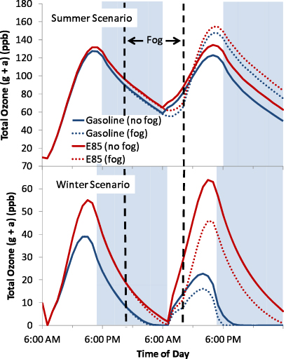
Figure 1. Two day total ozone (gas+aqueous) results for gasoline and E85 without a fog and with a fog for the summer scenario and the winter scenario.
Download figure:
Standard imageHowever, ozone increases in the afternoon after the morning fog in the summer for both gasoline and E85 compared with if no fog appears. To the contrary, ozone is lower after the fog in comparison with the no fog case in the winter (figure 1). Higher ozone after a fog has been observed in Shanghai where the highest values of maximum and mean ozone concentrations during a study were on a clear day with a heavy morning fog (Xu and Zhu 1994). Xu and Zhu (1994) hypothesize that the high ozone concentrations are due to either intensified vertical turbulence during and after the fog development or because it was a warm clear day after the fog. In our case, however, the increase in maximum ozone concentration on the warm days with a fog must have been due to aqueous chemistry. Through an analysis of species that impact the formation and reduction of O3, we found that the increase in peroxy radicals (RO2) during the morning fog in the summer scenario correlated the most with the increase in ozone (table S17 available at stacks.iop.org/ERL/7/045901/mmedia). The peroxy radicals do not increase during the fog in the winter scenario (table S18 available at stacks.iop.org/ERL/7/045901/mmedia). We tested the winter scenario using summer conditions for photolysis, temperature, and water vapor individually and found that the warm summer air increased the peroxy radicals for the winter gasoline case only and therefore increased ozone in the afternoon for the gasoline winter emissions case. The other cases (summer photolysis, summer water vapor, and the E85 case with summer temperatures for winter emissions) did not have an increase in peroxy radicals, and ozone decreased in the fog cases compared to the no fog cases, indicating that the mix of species being emitted is also a factor in ozone production.
The concentrations of several important species were averaged over the two day model run to facilitate comparisons of gasoline and E85 in the no fog and fog cases (figures S16 and S17 available at stacks.iop.org/ERL/7/045901/mmedia). The average ozone concentration increases by ∼7 ppb in the summer scenario and ∼16 ppb in the winter scenario without a fog when gasoline vehicles are replaced by flex-fuel vehicles running on E85. These results are similar to previous results (Ginnebaugh et al 2010), with slight differences due to small changes in the modeling conditions (deposition and ventilation were added here). The E85 minus gasoline differences decrease to ∼5.8 ppb and ∼11.2 ppb, respectively, when a morning fog is present. The relatively large increase in ozone in the winter (144% no fog, 114% with a fog) could be a concern for human health in cities with low temperatures and a high nitrogen oxide (NOx) to non-methane organic gases (NMOG) ratio. Ozone is typically low in cold climates and therefore not a concern. However, the increase in ozone concentrations with E85 may be significant enough that it would exceed 35 ppb, the threshold mixing ratio above which short-term health effects occur (Ostro et al 2006). Even small increases in ozone above the threshold, like observed in the warm temperature scenario, causes additional asthma, mortality, and hospitalizations due to respiratory illnesses. Increased risk of mortality due to short-term exposure to ozone is estimated to be 0.0004 ppb−1 above the threshold (Ostro et al 2006).
E85 increases peroxy acetyl nitrate (PAN), which damages crops and is a respiratory and eye irritant, by ∼0.7 ppb in the summer scenario and ∼2.8 ppb in the winter scenario without a fog (figures S16 and S17 available at stacks.iop.org/ERL/7/045901/mmedia). With a fog, the summer differences between E85 and gasoline are similar to the no fog case and the winter differences are smaller (∼2.2 ppb). Although PAN does not dissolve in the fog droplets in the model, its concentration is impacted by the fog through other dissolving species removed from the gas phase.
Average nitrogen oxide (NO) and nitrogen dioxide (NO2) concentrations decreased upon the switch to E85 by 8% and 13%, respectively, without a fog and 6% and 11%, respectively, with a fog for the summer scenario. The results differ for the winter scenario, with NO and NO2 reductions of 52% and 13% without a fog and 57% and 3% with a fog. Formaldehyde, acetaldehyde, acetic acid, and ethanol average concentrations all increase with E85. Formaldehyde and acetaldehyde are a concern because they are carcinogenic and acetic acid is a lung and eye irritant. Ethanol is a precursor to acetaldehyde. The fog affects the concentrations of gasoline and E85 cases differently. Figures 2 and S18 (available at stacks.iop.org/ERL/7/045901/mmedia) show how the fog impacts the average concentration for select species for the summer and winter scenarios. The average ozone concentration for the gasoline case is more strongly impacted by the fog (10% change) than for the E85 case (7% change) for the summer scenario, while the opposite is true for the winter scenario, where the change is −12% and −23%, respectively. It is not surprising that these changes differ from gasoline to E85 because the gas- and aqueous-phase chemistry are nonlinear and the mix of emissions differ. PAN increases by <1% for the gasoline and E85 cases with the fog in the summer and decreases by −2% and −4%, respectively, in the winter. NO2 decrease during the night with a fog due to scavenging of N2O5 (Lelieveld and Crutzen 1991), causing a general decrease in NOx in the summer scenario. In the winter scenario, NO concentrations increase during the fog and NO2 concentrations increase after the fog in the E85 case while remaining lower in the gasoline case (figures S12–S15 available at stacks.iop.org/ERL/7/045901/mmedia). The fog increases the average concentrations of formaldehyde but has little impact on the average concentrations of acetaldehyde, acetic acid, and ethanol on a per cent change basis. However, the average concentration only tells part of the story. For example, acetaldehyde decreases during the fog and increases after the fog (figure S8 available at stacks.iop.org/ERL/7/045901/mmedia), so although the average is similar between the no fog case and the fog case, the timing of the higher acetaldehyde concentrations differs.
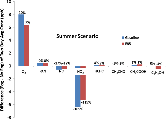
Figure 2. Difference (fog−no fog) and per cent change ((fog−no fog)/no fog) of two day average concentration (gas+aqueous) for select species for gasoline and E85 with the summer scenario.
Download figure:
Standard imageEthene has been found to be an important air pollutant with ethanol fuels (Gaffney et al 2012). Although it is fairly water soluble, it is not included in CAPRAM and the impact of fog on ethene is not investigated here.
The pH of the fog was allowed to vary during the simulation. The average pH of the fog was 2.69 and 2.71 for the gasoline and E85 cases, respectively, for the summer scenario (table S19 available at stacks.iop.org/ERL/7/045901/mmedia). The average pH was 4.82 and 3.23, respectively, for the winter scenario (table S20 available at stacks.iop.org/ERL/7/045901/mmedia). These are all in the range of pH's observed in fog droplets in the urban environment (Waldman et al 1982, Munger et al 1983, Jacob et al 1985, Munger et al 1990). These acidic fogs, for both gasoline and ethanol, negatively impact human health through inhalation (Hackney et al 1989, Laube et al 1993, Leduc et al 1995). The primary species to influence the pH of the fog was nitric acid (HNO3), shown in figures 3 and S19 (available at stacks.iop.org/ERL/7/045901/mmedia). Other top aqueous species in the fog include dissociated sulfuric acid, ammonium, oxygen, hydrochloric acid, glyoxal, formaldehyde, glycoaldehyde, methylglyoxal, and carbon dioxide.
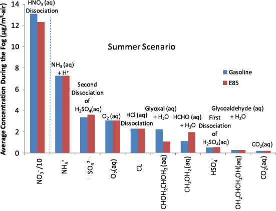
Figure 3. Average concentration of the top ten highest concentration aqueous species during the fog for the summer scenario (Note: NO3− is reduced by a factor of 10).
Download figure:
Standard imageAfter the fog evaporates, particulate matter (PM) remains. Some aqueous species return to the gas phase while others remain in the PM. In the summer scenario, nitric acid remains the top average aqueous species in the PM after the fog disappeared (figure S20 available at stacks.iop.org/ERL/7/045901/mmedia). For the winter scenario, hydrolyzed formaldehyde is on average the most abundant species in the PM (figure S21 available at stacks.iop.org/ERL/7/045901/mmedia). Tables S19 and S20 (available at stacks.iop.org/ERL/7/045901/mmedia) show that the majority of the average aqueous organic mass is single or double carbon species, both during and after the fog for summer and winter scenarios. The aqueous organic mass percentage of total aqueous species ranges from ∼3% during and after the fog for the summer scenario to 58% after the fog for the winter gasoline case. The summer aqueous species are dominated by nitric acid, whereas organic species are a larger share in the winter scenario.
The potential increases in pollutant concentration with E85 shown here should be considered when policy is being developed for the use of both ethanol and gasoline fuels to continue to improve air quality in US cities and keep ozone levels below the NAAQS (EPA 2011) and to reduce the health impacts of urban fog droplets (Hackney et al 1989, Laube et al 1993, Leduc et al 1995).
5. Sensitivity
The sensitivity of the no fog scenario to mixing height, water vapor, initial background conditions for NOx and NMOGs, total background emissions, and background emissions of NOx and toluene are discussed in detail in Ginnebaugh et al (2010). In all cases except where all background emissions were removed for the summer scenario, average ozone concentrations were higher using E85 instead of gasoline (Ginnebaugh et al 2010).
Here, we investigate the impact of different fog parameters on the ozone results. Table 1 lists the sensitivity cases and the changes made to the fog for each case. For the summer scenario, reducing the droplet size reduced ozone by 3% while making almost no change in the winter scenario, as shown in figures 4 and S22 (available at stacks.iop.org/ERL/7/045901/mmedia). The mass transfer coefficient for species from the gas to the aqueous phases is proportional to the droplet radius, so a smaller droplet size would reduce transfer from the gas phase to the aqueous phase. This reduces the peroxy radical (RO2) production in the aqueous phase which lowers ozone production after the fog has dissipated in the summer scenario. In the winter scenario, peroxy radical production is already lower in the fog case and a reduction in droplet size only reduces ozone concentrations slightly.

Figure 4. Difference in two day average ozone (gas+aqueous) concentration (sensitivity−baseline fog case) and per cent change ((sensitivity−baseline fog)/baseline fog) to test the model's sensitivity to fog parameters for the summer scenario.
Download figure:
Standard imageTable 1. List of fog parameters for each fog sensitivity case .
| Fog sensitivity case | LWC (cm3-water/cm3-air) | Droplet diameter (μm) | Photolysis reduction during fog/aerosol (%) | Duration of fog/aerosol |
|---|---|---|---|---|
| Baseline fog | 3.0 × 10⁻⁷ | 20 | 30 | 10 pm to 10 am |
| Smaller drop | 3.0 × 10⁻⁷ | 10 | 30 | 10 pm to 10 am |
| Aerosol | 2.5 × 10⁻¹⁰ | 0.5 | 30 | 10 pm to 10 am |
| Lower LWC | 1.0 × 10⁻⁸ | 20 | 30 | 10 pm to 10 am |
| Higher LWC | 5.0 × 10⁻⁷ | 20 | 30 | 10 pm to 10 am |
| Longer duration fog | 3.0 × 10⁻⁷ | 20 | 30 | 10 pm to 2 pm |
| Decreased photolysis | 3.0 × 10⁻⁷ | 20 | 60 | 10 pm to 10 am |
| No photolysis reduction (fog) | 3.0 × 10⁻⁷ | 20 | 0 | 10 pm to 10 am |
| No photolysis reduction (aerosol) | 2.5 × 10⁻¹⁰ | 0.5 | 0 | 10 pm to 10 am |
Lower liquid water content (aerosol and lower LWC cases) increases average ozone by 3–4% in the summer and 4–23% in the winter scenarios. Higher liquid water content (higher LWC case) has the opposite effect. The liquid water content is directly proportional to the dissolution rate and aqueous oxidation rates, so lower liquid water content decreases ozone scavenging by the fog.
A longer fog duration and a thicker fog (less sunlight) both decrease average ozone in summer and winter (longer duration fog and decreased photolysis cases). A thin fog or an aerosol layer that does not reduce photolysis rates increases average ozone (no photolysis reduction cases). In all fog sensitivity cases, the average ozone from the E85 case was higher than the average ozone from the gasoline case.
6. Conclusion
We find here that, when considering photochemistry alone, E85 increases ozone slightly compared with gasoline in the presence or absence of a fog under summer conditions but increases ozone relative to gasoline much more during winter conditions, although winter ozone is lower than summer ozone for both gasoline and E85. This result supports previous work that has found that E85 is no better than gasoline for ozone formation and carcinogenic species and is not a 'clean-burning' fuel (Jacobson 2007, Gaffney and Marley 2009, Cook et al 2011). A new finding here is that a morning fog during summer can increase ozone after the fog due to chemistry alone. A morning fog on a winter day decreases ozone after the fog. The acidity of the fog is similar between E85 and gasoline in the summer but more acidic for E85 in the winter. Peroxy acetyl nitrate (PAN) levels increase in both summer and winter with E85, but more in winter, relative to gasoline.
Acknowledgments
The authors would like to thank Hartmut Herrmann and Andreas Tilgner for providing information and assistance related to CAPRAM. This work was supported by the US Environmental Protection Agency grant RD-83337101-O and the National Science Foundation.