
Abstract
Recent studies have examined tropical upper tropospheric warming by comparing coupled atmosphere–ocean global circulation model (GCM) simulations from Phase 3 of the Coupled Model Intercomparison Project (CMIP3) with satellite and radiosonde observations of warming in the tropical upper troposphere relative to the lower-middle troposphere. These studies showed that models tended to overestimate increases in static stability between the upper and lower-middle troposphere. We revisit this issue using atmospheric GCMs with prescribed historical sea surface temperatures (SSTs) and coupled atmosphere–ocean GCMs that participated in the latest model intercomparison project, CMIP5. It is demonstrated that even with historical SSTs as a boundary condition, most atmospheric models exhibit excessive tropical upper tropospheric warming relative to the lower-middle troposphere as compared with satellite-borne microwave sounding unit measurements. It is also shown that the results from CMIP5 coupled atmosphere–ocean GCMs are similar to findings from CMIP3 coupled GCMs. The apparent model-observational difference for tropical upper tropospheric warming represents an important problem, but it is not clear whether the difference is a result of common biases in GCMs, biases in observational datasets, or both.
Export citation and abstract BibTeX RIS

Content from this work may be used under the terms of the Creative Commons Attribution-NonCommercial-ShareAlike 3.0 licence. Any further distribution of this work must maintain attribution to the author(s) and the title of the work, journal citation and DOI.
1. Introduction
A robust feature of GCM simulations of the 21st century climate is enhanced tropical upper tropospheric warming with temperature trends increasing as a function of height until about 200 hPa (IPCC 2007). This characteristic accounts for much of the lapse rate and associated water vapor feedbacks in GCMs, which are important factors for climate sensitivity (e.g. Soden and Held 2006). Vertical amplification of tropical tropospheric temperature trends relative to surface trends has been examined in a number of studies and there is strong evidence that no serious inconsistency exists between GCMs and observations (e.g. Fu et al 2004, Fu and Johanson 2005, Santer et al 2005, Thorne et al 2007, Santer et al 2008), though some studies find otherwise (e.g. Christy et al 2007, Douglass et al 2008, Christy et al 2010). Recent studies of temperature trend amplification in the tropical upper troposphere relative to the lower-middle troposphere found that coupled atmosphere–ocean models from CMIP3 exaggerated this amplification compared to satellite microwave sounding unit (MSU) (Fu et al 2011) and radiosonde (Seidel et al 2012) observations.
A confounding factor in comparing coupled atmosphere–ocean GCMs with observations is that coupled GCM's internally generated natural variability is not the same as the observational record. Furthermore, historical simulations from coupled GCMs have larger tropical tropospheric temperature trends compared to observations since 1979 (Fu et al 2011). Fu et al (2011) demonstrated that some of the differences in the change of static stability between the tropical upper and lower-middle troposphere between models and observations are a result of an overestimation of tropical warming in CMIP3 coupled GCM simulations. This study utilizes CMIP5 model simulations (Taylor et al 2012) from the Atmospheric Model Intercomparison Project (AMIP). AMIP model simulations use observational records of sea ice and SST evolution (e.g. Hurrell et al 2008) as boundary conditions for atmospheric GCMs. Thus the AMIP model's SSTs have the same variability and trends as observations. Previous studies have demonstrated that AMIP style runs can closely reproduce the observed tropical tropospheric temperature variations (Hurrell and Trenberth 1997). The use of AMIP models allows us to closely examine simulated changes of the vertical temperature structure in the tropical troposphere in GCMs using the observed SST evolution.
Another advantage of the AMIP simulations is that the spatial pattern of SST changes in the models is constrained to the observations, which may affect tropical tropospheric amplification. Deep convection typically occurs over warm tropical SST regions (e.g. Wallace 1992, Johnson and Xie 2010), which act as a heating source for the tropical free troposphere. This large-scale heating occurs because any anomalous heating is quickly distributed in the tropics, which do not maintain strong horizontal temperature gradients (e.g. Bretherton and Sobel 2003). The tropical mean tropospheric temperature profile should roughly follow a moist adiabat that is determined by warmest SST regions (e.g. Sobel et al 2002). As a result, the specific pattern of SST warming could affect the structure of the temperature change in the tropical troposphere. Using AMIP models in this study will ensure that the effect of the pattern of SST changes on disagreements between models and observations is minimized.
In this letter, observed changes in the temperature structure of the tropical troposphere from MSU observations are compared to changes in CMIP5 models. This work will concentrate on GCMs constrained with observed SSTs, referred to as AMIP models throughout this letter. We will also update Fu et al (2011) by comparing coupled atmosphere–ocean 'historical' runs from CMIP5 (Fu et al (2011) used CMIP3 models). Coupled atmosphere–ocean model experiments that do not constrain SSTs with observations will be referred to as coupled models. Broadly, CMIP5 refers to the most recent international GCM intercomparison project, from which we will utilize AMIP model simulations (model simulations constrained by observed SSTs) and coupled models (models that fall under the 'historical' experiment that are not constrained by observed SSTs). The main focus of this research is to determine if model and observational discrepancies seen in Fu et al (2011) and Seidel et al (2012) can be reconciled in atmospheric models using prescribed historical SSTs (i.e. AMIP models). We show that even by constraining atmospheric models with prescribed SSTs, model upper tropospheric warming relative to the lower-middle troposphere is still significantly larger than observations for most models. We also show that the results for CMIP5 coupled model simulations are similar to CMIP3 results (Fu et al 2011).
2. MSU datasets and model simulations
The MSU and its successor, the advanced MSU (AMSU), have provided global temperature measurements of deep atmospheric layers since late 1978. Because MSU and AMSU instruments have flown onboard a number of satellites, their temperature records have been combined into a single, continuous, homogenized climate record. In this work, we will utilize two datasets that have been created to remove the influence of the stratosphere. The lower-middle tropospheric channel, TLT, utilizes a linear combination of view angles from the mid-tropospheric channel, T2, with a weighting function that peaks near 600 hPa (Spencer and Christy 1992). Another derived temperature dataset uses observations from the lower stratospheric channel, T4, to remove the influence of the stratosphere on T2 (Fu et al 2004, Johanson and Fu 2006). This dataset, referred to as T24, has a weighting function that peaks near 300 hPa and represents the upper-middle troposphere. We will combine MSU T2 and T4 observations to produce a T24 time series using a tropical weighting of T24 = 1.1T2 − 0.1T4 (Johanson and Fu 2006). This study will utilize gridded monthly TLT and T24 data to compute a tropical mean (20°S–20°N) time series. We will then use the T24–TLT trend and the ratio of T24 to TLT trends as metrics to determine the relative temperature amplification between the upper troposphere and the lower-middle troposphere following Fu et al (2011). Note that T24–TLT effectively compares the temperature of a layer between 100 and 500 hPa (with a maximum weighting near 200 hPa) with the temperature for a layer between 500 hPa and the surface (see figure 1 in Fu et al 2011). The T24–TLT difference therefore represents the difference between the tropical upper troposphere and the lower-middle troposphere. Throughout this letter, we refer to TLT and T24 deep layer measurements as measurements of the lower-middle and upper-middle troposphere, respectively, since the weighting functions for these datasets are broad. In referring to the difference between these datasets, we use the terminology upper to lower-middle troposphere, since the difference weighting function has a sharper peak in the upper troposphere.
Our T24 and TLT MSU observations come from the University of Alabama in Huntsville (UAH) and Remote Sensing Systems (RSS). The National Oceanographic and Atmospheric Administration (NOAA) also provides observations for T2 and T4, which allow us to create a T24 time series, but NOAA does not currently produce a TLT product. We will use RSS v3.3 (Mears and Wentz 2009a, 2009b), UAH v5.4 (Christy et al 2003) and NOAA STAR v2.0 (Zou and Wang 2011). All of the teams that produce MSU products account for a number of non-climatic biases such as satellite orbital decay, contamination related to the satellite warm target calibration, and drift in the local sampling time of the satellite (e.g. Fu and Johanson 2005, Mears and Wentz 2005, CCSP 2006, Wentz and Schabel 1998, Christy et al 2000, Po-Chedley and Fu 2012). As a result of the different procedures for bias removal, the various teams derive different long-term temperature trends for TLT and T24, but the relative warming in TLT compared to T24 is consistent for both UAH and RSS, likely because each group uses similar bias removal procedures for each of its own channels.
We will compare GCMs in the CMIP5 archive to MSU observations. Specifically, we will utilize models that contributed coupled 'historical' simulations (44 models) and models that contributed AMIP simulations (19 models). Taylor et al (2012) provides more details on the CMIP5 experimental design. In both experiments, the atmospheric composition evolves in the model to reflect natural and anthropogenic forcings, but the atmospheric changes are not the same across all models. For example, not all models include emissions from volcanic eruptions. Hurrell and Trenberth (1997) noted that even when volcanic forcings are not included in atmospheric models, most of their influence is captured by the SST forcing. In order to compare the model simulations to satellite observations, we apply a static weighting function (from RSS) to the model's tropical (20°S–20°N) monthly mean temperature profile to produce an MSU equivalent brightness temperature time series.
3. Temperature trend difference between the tropical upper and lower-middle troposphere
Figure 1 shows the time evolution of TLT for both coupled and AMIP model simulations and MSU satellite observations. The model spread is dramatically reduced in the AMIP models owing to the prescribed observational SSTs, and there is good agreement between the multi-model mean and the observed average (i.e., the average of RSS and UAH) TLT time series (r = 0.89 for 1979–2008). There is noticeable disagreement between AMIP models and MSU observations in 1979 and 1980 (the r-value improves to 0.92 for 1981–2008). This disagreement has been discussed in the past and it is unclear if the disagreement is an artifact of the SST datasets used by the AMIP models, the MSU datasets, a problem with the models, or some combination of these factors (Hurrell and Trenberth 1997, 1998, Christy et al 1997, 1998). To avoid this time period, we begin our analysis in 1981, but we note that including these years increases the disagreement between modeled and observed measurements of the T24–TLT trend. The coupled historical models are listed in table 1 and the AMIP models are listed in table 2. In tables 1 and 2, we also include the model ensemble mean trend values for TLT, T24 and T24–TLT, and the ratio of T24 to TLT trends. Note that we used the time period 1981–2005 for the coupled models, because many of the coupled models only extend through 2005. The AMIP models used in this letter all extend through 2008, which allows us to use the time period 1981–2008. The AMIP models have trend values that are in much better agreement with the observations, but the amplification ratio (i.e. the ratio of the T24 to TLT trend) is larger for both coupled and AMIP GCMs compared to the MSU observations. There is only one instance in which a model ensemble mean has a lower amplification ratio than the MSU observations. As a whole, the trend amplification ratio in both AMIP and coupled GCMs is ∼1.2, which represents an increase in static stability between the tropical upper troposphere and the lower-middle troposphere.
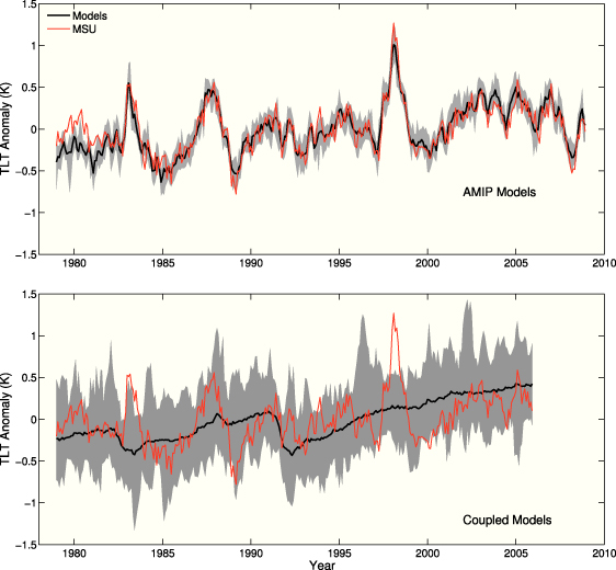
Figure 1. Times series of TLT monthly temperature anomalies in the tropics (20°S–20°N) for AMIP GCM (top) and coupled GCM (bottom) simulations (black) and the average of RSS and UAH (red). The model spread is shaded. Many coupled GCM simulations only extended to 2005, while AMIP runs included here extended to 2008.
Download figure:
Standard imageTable 1. Trend values for TLT and T24 in K decade−1 from the MSU teams and the ensemble mean of each coupled climate model (CMIP5 historical simulations). The trends are the simple mean of the TLT, T24, and T24–TLT trends of all of the ensemble members for each model. The ratio is the average T24 trend divided by the average TLT trend. The trends are for the tropics (20°S–20°N) over the period 1981–2005. Trend values of T24–TLT are in units of K decade−1 and the ratio of T24 to TLT trends are also given as a measure of the vertical temperature trend amplification in the tropical troposphere.
| TLT | T24 | T24–TLT | Ratio | |
|---|---|---|---|---|
| UAH | 0.118 | 0.129 | 0.011 | 1.09 |
| RSS | 0.203 | 0.222 | 0.020 | 1.10 |
| NOAA | n/a | 0.265 | n/a | n/a |
| ACCESS1.0 | 0.316 | 0.375 | 0.059 | 1.19 |
| ACCESS1.3 | 0.227 | 0.260 | 0.033 | 1.14 |
| BCC-CSM1.1 | 0.274 | 0.317 | 0.043 | 1.16 |
| BCC-CSM1.1 (m) | 0.318 | 0.376 | 0.059 | 1.19 |
| BNU-ESM | 0.261 | 0.314 | 0.053 | 1.20 |
| CanCM4 | 0.283 | 0.337 | 0.054 | 1.19 |
| CanESM2 | 0.336 | 0.398 | 0.062 | 1.18 |
| CCSM4 | 0.287 | 0.345 | 0.058 | 1.20 |
| CESM1(BGC) | 0.219 | 0.266 | 0.047 | 1.21 |
| CESM1(CAM5) | 0.247 | 0.297 | 0.050 | 1.20 |
| CESM1(CAM5.1,FV2) | 0.187 | 0.226 | 0.039 | 1.21 |
| CESM1(FASTCHEM) | 0.255 | 0.307 | 0.051 | 1.20 |
| CESM1(WACCM) | 0.279 | 0.332 | 0.053 | 1.19 |
| CMCC-CM | 0.236 | 0.291 | 0.054 | 1.23 |
| CNRM-CM5 | 0.229 | 0.250 | 0.021 | 1.09 |
| CSIRO-Mk3.6.0 | 0.241 | 0.284 | 0.043 | 1.18 |
| EC-EARTH | 0.240 | 0.272 | 0.032 | 1.13 |
| FGOALS-g2 | 0.223 | 0.260 | 0.036 | 1.16 |
| FGOALS-s2 | 0.274 | 0.319 | 0.045 | 1.16 |
| FIO-ESM | 0.241 | 0.292 | 0.050 | 1.21 |
| GFDL-CM2.1 | 0.398 | 0.464 | 0.066 | 1.16 |
| GFDL-CM3 | 0.364 | 0.435 | 0.071 | 1.20 |
| GFDL-ESM2G | 0.452 | 0.522 | 0.070 | 1.15 |
| GFDL-ESM2M | 0.319 | 0.374 | 0.055 | 1.17 |
| GISS-E2-H | 0.271 | 0.320 | 0.049 | 1.18 |
| GISS-E2-R | 0.266 | 0.316 | 0.051 | 1.19 |
| HadCM3 | 0.290 | 0.342 | 0.052 | 1.18 |
| HadGEM2-AO | 0.335 | 0.390 | 0.055 | 1.16 |
| HadGEM2-CC | 0.245 | 0.284 | 0.039 | 1.16 |
| HadGEM2-ES | 0.252 | 0.296 | 0.044 | 1.18 |
| INM-CM4 | 0.100 | 0.120 | 0.020 | 1.20 |
| IPSL-CM5A-LR | 0.404 | 0.487 | 0.083 | 1.21 |
| IPSL-CM5A-MR | 0.341 | 0.417 | 0.075 | 1.22 |
| IPSL-CM5B-LR | 0.287 | 0.356 | 0.069 | 1.24 |
| MIROC-ESM | 0.153 | 0.195 | 0.042 | 1.28 |
| MIROC-ESM-CHEM | 0.083 | 0.117 | 0.034 | 1.42 |
| MIROC4h | 0.363 | 0.437 | 0.074 | 1.20 |
| MIROC5 | 0.190 | 0.227 | 0.037 | 1.20 |
| MPI-ESM-LR | 0.362 | 0.421 | 0.060 | 1.17 |
| MPI-ESM-MR | 0.325 | 0.384 | 0.058 | 1.18 |
| MPI-ESM-P | 0.296 | 0.348 | 0.052 | 1.18 |
| MRI-CGCM3 | 0.194 | 0.229 | 0.036 | 1.18 |
| NorESM1-M | 0.222 | 0.263 | 0.040 | 1.18 |
| NorESM1-ME | 0.257 | 0.307 | 0.049 | 1.19 |
| Model average | 0.271 | 0.322 | 0.051 | 1.19 |
Table 2. As in table 1 but for the MSU teams and CMIP5 AMIP GCM simulations over the period 1981–2008.
| TLT | T24 | T24–TLT | Ratio | |
|---|---|---|---|---|
| UAH | 0.082 | 0.086 | 0.004 | 1.05 |
| RSS | 0.149 | 0.164 | 0.015 | 1.10 |
| NOAA | n/a | 0.205 | n/a | n/a |
| BCC-CSM1.1 | 0.166 | 0.192 | 0.027 | 1.16 |
| CanAM4 | 0.174 | 0.216 | 0.042 | 1.24 |
| CCSM4 | 0.176 | 0.217 | 0.042 | 1.24 |
| CNRM-CM5 | 0.184 | 0.209 | 0.025 | 1.14 |
| FGOALS-s2 | 0.171 | 0.207 | 0.036 | 1.21 |
| GFDL-HIRAM-C180 | 0.140 | 0.158 | 0.018 | 1.13 |
| GFDL-HIRAM-C360 | 0.143 | 0.165 | 0.022 | 1.15 |
| GISS-E2-R | 0.136 | 0.154 | 0.018 | 1.13 |
| HadGEM2-A | 0.173 | 0.199 | 0.026 | 1.15 |
| INM-CM4 | 0.155 | 0.187 | 0.032 | 1.21 |
| IPSL-CM5A-LR | 0.163 | 0.200 | 0.037 | 1.23 |
| IPSL-CM5B-LR | 0.167 | 0.203 | 0.037 | 1.22 |
| MIROC5 | 0.184 | 0.226 | 0.043 | 1.23 |
| MPI-ESM-LR | 0.191 | 0.230 | 0.039 | 1.20 |
| MPI-ESM-MR | 0.190 | 0.225 | 0.035 | 1.19 |
| MRI-AGCM3.2H | 0.131 | 0.157 | 0.026 | 1.20 |
| MRI-AGCM3.2S | 0.130 | 0.159 | 0.029 | 1.22 |
| MRI-CGCM3 | 0.171 | 0.209 | 0.038 | 1.22 |
| NorESM1-M | 0.174 | 0.213 | 0.039 | 1.22 |
| Model average | 0.164 | 0.196 | 0.032 | 1.19 |
Since AMIP models are constrained by observed SSTs, it is possible to closely compare the time evolution of the upper tropospheric warming between models and observations using the difference between the upper-middle and lower-middle tropospheric temperatures (i.e. T24–TLT). Figure 2 shows the trend of the difference time series between AMIP simulations and observations for T24–TLT (i.e. (T24–TLT)AMIP − (T24–TLT)MSU). In figure 2 we see that most models have T24–TLT trends that significantly exceed MSU observations with 95% confidence. The ensemble mean of every model has larger T24–TLT trends than observations. 17 (12) of the 19 models have significantly greater T24–TLT trends than UAH (RSS) with 95% confidence. Even though GCMs generally have larger T24–TLT trends than MSU observations, the GFDL and GISS models show good agreement with RSS. Note that figure 2 in this work is different from figure 2 in Fu et al (2011) where the trends of T24–TLT were shown. In Fu et al (2011) the trend for (T24–TLT)COUPLED was compared with the trend for (T24–TLT)MSU using a two-sample t-test (Lanzante 2005) to determine if the (T24–TLT)COUPLED trend was statistically different from the (T24–TLT)MSU trend.
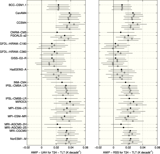
Figure 2. Trend of the differences between AMIP simulations and observations for T24–TLT over 1981–2008 for UAH (left) and RSS (right) in the tropics (20°S–20°N) (i.e., the trend of (T24–TLT)AMIP − (T24–TLT)MSU). Open circles are individual AMIP model ensemble members and the solid circles represent the ensemble mean for a given AMIP model. The error bars represent the 95% confidence interval, including the effects of autocorrelation.
Download figure:
Standard imageWe also repeated the analysis from Fu et al (2011), comparing the T24–TLT trends in coupled GCMs and satellites over the period 1981–2005. As can be seen from table 1, the results shown here for CMIP5 coupled models are similar to the CMIP3 models in Fu et al (2011), but using the newer CMIP5 simulations. The upper tropospheric warming relative to the lower-middle troposphere is consistently larger in models than observations. The T24–TLT ensemble mean trends from all but one CMIP5 coupled GCM are significantly larger than zero while T24–TLT trends from both UAH and RSS are not significantly different from zero (not shown here). Even though we use a shorter time period than Fu et al (2011), 27 (15) of the 44 models have trends that are significantly different from UAH (RSS) using two-sample t-tests (Lanzante 2005). One reason that a smaller fraction of models are significantly different from MSU data compared to Fu et al (2011) is because we use seven fewer years, which decreases the number of degrees of freedom and increases the uncertainty in the trend for both models and observations. Another reason that some coupled models are not significantly different from observations is that coupled models often overestimate the interannual variability, which increases the model trend error. No model has an ensemble mean T24–TLT trend as low as RSS or UAH (table 1). We also note from table 1 that CMIP5 coupled GCMs largely overestimate tropical warming just as CMIP3 models overestimated tropical warming (Fu et al 2011).
Figure 3 demonstrates the distribution of T24 to TLT trend ratios in AMIP simulations. AMIP models consistently have larger ratios than MSU observations, even though the models are constrained with observed SSTs. Of the 55 ensemble members, all have trend amplification ratios exceeding that of UAH, and only two ensemble members have less amplification than RSS. In the coupled historical simulations only 5 (6) ensemble members of 185 have amplification ratios less than UAH (RSS), and they are all from the same model (CNRM-CM5). Figure 4 demonstrates the scaling of interannual and decadal amplification for the tropical upper-middle troposphere relative to the lower-middle troposphere. The decadal amplification is the ratio of the T24 trend to the TLT trend, while the interannual amplification is the standard deviation of the de-trended monthly T24 anomaly time series divided by the standard deviation of the de-trended monthly TLT anomaly time series. The decadal amplification is a measure of the upper- to lower-middle tropospheric temperature amplification over the past ∼3 decades, whereas the interannual amplification is a measure of the amplification on interannual time scales. It is striking that even though the interannual amplification of UAH and RSS is in the range of the model results, both show less decadal amplification compared to the models. Figures 3 and 4 suggest that models consistently have greater vertical temperature trend amplification between the tropical upper- to lower-middle troposphere compared to satellite MSU observations, even though the amplification in models has a large range.
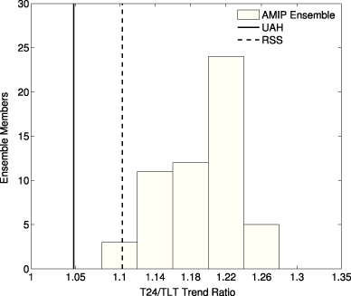
Figure 3. Histogram of the ratio of the T24 trend to the TLT trend over 1981–2008 from AMIP ensemble members in the tropics (20°S–20°N). The T24 to TLT trend ratios for RSS and UAH are shown for comparison. The T24/TLT trend ratios under the histogram bins represent the bin center values.
Download figure:
Standard image
Figure 4. Decadal versus interannual amplification of T24 to TLT from both AMIP and coupled GCM simulations and MSU observations in the tropics (20°S–20°N) between 1981 and 2005. The decadal amplification is defined as the T24 trend divided by the TLT trend. The interannual amplification is defined as the standard deviation of the de-trended monthly T24 anomaly time series divided by the standard deviation of the de-trended monthly TLT anomaly values. Each cross or circle represents the ensemble mean for each model. The mean of all models is given by the bold symbols. Note that the MIROC-ESM-CHEM model is not contained in this plot as it has a relatively large decadal amplification value (table 1), likely related to biases after the Mt. Pinatubo eruption in 1991 (Watanabe et al 2011).
Download figure:
Standard image4. Discussion and conclusions
We have demonstrated that GCMs typically exhibit greater tropical upper to lower-middle tropospheric amplification compared to satellite-borne deep layer temperature observations for both coupled historical simulations and simulations constrained with historical SSTs. For most of the AMIP models, the relative warming in the upper troposphere compared to the lower-middle troposphere is significantly (95% confidence) larger than both RSS and UAH, but some models such as GFDL and GISS demonstrate good agreement with RSS.
There are a number of explanations for the differences in tropical upper to lower-middle tropospheric temperature trend amplification. The consistent positive bias (though not always significant) in models for T24–TLT trends or T24/TLT trend ratios as compared to both UAH and RSS indicates that this might be a common problem amongst models. In figure 5, we demonstrate the relationship between the annual mean tropical (20°S–20°N) T24 temperature and the ratio of the T24 trend to the TLT trend for AMIP models over 1981–2008. The relationship between the annual mean T24 temperature and the upper- to lower-middle tropospheric amplification is significant (95% confidence) with r = 0.56. One possible explanation for this relationship is that model parameterizations (i.e. deep convection, radiation or clouds) that influence the mean state climate have important implications for the changes in the static stability between the tropical upper and lower-middle troposphere. John and Soden (2007) found that CMIP3 coupled models tended to have cold biases in the tropical troposphere relative to reanalysis models and AIRS satellite infrared measurements and that these biases had little effect on the model's lapse rate and water vapor feedbacks on a global scale. Note that John and Soden (2007) considered the total column global mean tropospheric biases. Although measuring climatological biases are outside the scope of this work, figure 5 does suggest that the simulated tropical upper-middle tropospheric climatology may be related to the magnitude of lapse rate changes between the tropical upper and lower-middle troposphere.
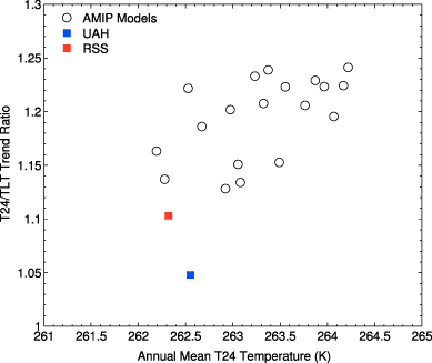
Figure 5. Decadal amplification (as in figure 4) versus the annual mean T24 temperature over 1981–2008 for AMIP models. The relationship is statistically significant (95% confidence) and the r-value is 0.56. The annual mean T24 temperatures are also presented for RSS and UAH for reference. Note that much of the focus for MSU groups has been on relative changes and not on absolute temperature calibration (e.g. Mears et al 2011).
Download figure:
Standard imageThe effect of internal uncertainty related to the dataset construction is large (Christy et al 2003, Zou et al 2009, Mears et al 2011), so it is possible that the differences between GCMs and observations are byproducts of the merging procedure for satellite observations. It is unclear why the interannual amplification ratio should be different from the decadal amplification ratio, but MSU observations show less amplification on decadal time scales (figure 4). We also note that NOAA T24 has larger upper-middle tropospheric warming compared to RSS and UAH (tables 1 and 2) and that other analyses that use temperature trends derived from wind measurements have found that historical tropical tropospheric warming is largely consistent with GCM results (Allen and Sherwood 2008). In general, the comparison of model and observed trends over a relatively short time period has large uncertainties, so some of the discrepancy noted here may also be related to the length of the datasets.
A further possibility is that the agreement with some models (i.e. GFDL and GISS) is real and the remaining models exhibit too much tropical upper to lower-middle tropospheric temperature trend amplification. With the latter possibility, it would be important to investigate why some atmospheric models exhibit too much amplification given that the representation of tropical upper to lower-middle tropospheric temperature trend amplification may be important to model estimates of climate sensitivity. In at least two cases, modeling groups (GFDL and NASA GISS) used a different SST dataset (HadISST, Rayner et al 2003) than that recommended for the CMIP5 AMIP experiment (Held and Ken Lo 2012). The GFDL and GISS models have tropical upper to lower-middle tropospheric amplification characteristics that agree much better with observations, indicating that the SST dataset may explain some of the discrepancies noted here.
Given the importance of both models and observations, it will be important to continue to investigate this discrepancy between models and observations. The representation of upper tropospheric warming in models is important to climate sensitivity and thus future projections of anthropogenic global warming. Furthermore, SST and MSU datasets represent vital records for monitoring climate change, so it is important to resolve any errors that may exist. At a more basic level, understanding the discrepancies highlighted here may help advance our understanding of the coupling between the atmosphere and the ocean in the tropics and its implications for climate change.
Acknowledgments
We would like to thank Drs Isaac Held, Syukuro Manabe and Dian Seidel for motivating and commenting on this research. We also thank two anonymous reviewers for their helpful comments. This work was supported by the National Science Foundation Graduate Research Fellowship (DGE-0718124), National Science Foundation of China under grant 41275070, DOE grant DE-FG02-09ER64769, and NOAA NESDIS-NESDISPO-2009-2001589 (SDS-09-15). We acknowledge the World Climate Research Programme's Working Group on Coupled Modeling, which is responsible for CMIP, and we thank the climate modeling groups (models are listed in tables 1 and 2 of this paper) for producing and making available their model output. For CMIP, the US Department of Energy's Program for Climate Model Diagnosis and Intercomparison provides coordinating support and led development of software infrastructure in partnership with the Global Organization for Earth System Science Portals.