
Abstract
The most up to date consensus from global climate models predicts warming in the Northern Hemisphere (NH) high latitudes to middle latitudes during boreal winter. However, recent trends in observed NH winter surface temperatures diverge from these projections. For the last two decades, large-scale cooling trends have existed instead across large stretches of eastern North America and northern Eurasia. We argue that this unforeseen trend is probably not due to internal variability alone. Instead, evidence suggests that summer and autumn warming trends are concurrent with increases in high-latitude moisture and an increase in Eurasian snow cover, which dynamically induces large-scale wintertime cooling. Understanding this counterintuitive response to radiative warming of the climate system has the potential for improving climate predictions at seasonal and longer timescales.
Export citation and abstract BibTeX RIS
1. Introduction
Global surface temperatures have generally warmed for the entire length of the instrumental record. The most significant and strongest warming occurred in the most recent 40 yr, with Arctic temperatures warming at nearly double the global rate (Solomon et al 2007, Screen and Simmonds 2010). Coupled climate models attribute much of this warming to rapid increases in greenhouse gases (GHGs) and project the strongest warming across the extratropical NH during boreal winter due to 'winter (or Arctic) amplification' (Holland and Bitz 2003, Hansen and Nazarenko 2004, Alexeev et al 2005, Langen and Alexeev 2007). Yet, while the planet has steadily warmed, NH winters have recently grown more extreme across the major industrialized centres. Record cold snaps and heavy snowfall events across the United States, Europe and East Asia garnered much public attention during the winters of 2009/10 and 2010/11 (Blunden et al 2011, Cohen et al 2010). Cohen et al (2009) argued that the occurrence of more severe NH winter weather is a two-decade-long trend starting around 1988. Whether the recent colder winters are a consequence of internal variability or a response to changes in boundary forcings resulting from climate change remains an open question.
In this letter, we propose that the extensive winter NH extratropical cooling trend amidst a warming planet cannot be explained entirely by internal variability of the climate system. It has been shown that above normal snow cover across Eurasia in the autumn leads to a negative Arctic Oscillation (AO) and cold temperatures across the eastern United States and northern Eurasia in winter (Cohen and Entekhabi 1999). Therefore, we suggest that a significant portion of the wintertime temperature trend is driven by dynamical interactions between October Eurasian snow cover, which has increased over the last two decades, and the large-scale NH extratropical circulation in the late autumn and winter.
2. Observational data and model output
Observational surface temperature data originate from three sources: (1) the Climate Research Unit land air temperature data set, version 3 (CRUTEM3; Brohan et al 2006); (2) the Modern-Era Retrospective Analysis for Research and Applications (MERRA; Rienecker et al 2011); and (3) the National Center for Environmental Protection (NCEP)/National Center for Atmospheric Research (NCAR) Reanalysis Project (Kalnay et al 1996). The CRUTEM3 consists of land-based temperature anomalies on a regular 5° × 5° longitude/latitude grid globally. MERRA temperatures reside on a 1.25° × 1.25° grid, and NCEP/NCAR reanalysis temperatures on a 2.5° × 2.5° grid. Only values over land for MERRA and NCEP/NCAR are used. For all data sets, we use the same time period (1988–2010). Monthly anomalies from MERRA and the NCEP/NCAR reanalysis fields are computed by removing the climatological monthly means from the raw data.
Lower tropospheric moisture over the Arctic is derived by vertically integrating specific humidity from MERRA from 1000 to 700 hPa and area-averaging the field poleward of 60°N. The Integrated Global Radiosonde Archive (Durre et al 2009, Elliott et al 2002) is also used to compute precipitable water (table 1). Daily data from soundings for all Octobers were stacked together and only stations with more than 80% available data were used. Both 00Z and 12Z times of radiosonde launch were used if data coverage was sufficient. Only one time was used if coverage in another one was poor in order to remove the potential influence of the diurnal cycle.
Table 1. List of radiosonde stations from the Integrated Global Radiosonde Archive used for precipitable water trends calculated and presented in figure 3. The location of the station and the time span of the record from each station are included.
| Station ID | Location | Latitude (°N) | Longitude (°E) | Time span |
|---|---|---|---|---|
| RS 20674 | Ostrov Dikson | 73.50 | 80.42 | 1948–2011 |
| RS 20891 | Khatanga | 71.98 | 102.47 | 1950–2011 |
| RS 21824 | Bukhta Tiksi | 71.63 | 128.85 | 1948–2011 |
| RS 21946 | Cokurdah | 70.62 | 147.88 | 1965–2011 |
| RS 23205 | Narian Mar | 67.65 | 53.02 | 1963–2011 |
| RS 23330 | Salekhard (Obdorsk) | 66.53 | 66.53 | 1948–2011 |
| RS 23472 | Turukhansk | 65.78 | 87.95 | 1963–2011 |
| RS 23884 | Podkamennaia-Tunguska | 61.60 | 90.00 | 1963–2011 |
| RS 23955 | Aleksandrovskoe | 60.43 | 77.87 | 1949–2011 |
| RS 24266 | Verkhoyansk | 67.55 | 133.38 | 1964–2011 |
| RS 24343 | Zhigansk | 66.77 | 123.40 | 1965–2011 |
| RS 24641 | Viliuysk | 63.77 | 121.62 | 1950–2011 |
| RS 24688 | Oimakon | 63.47 | 142.80 | 1950–2011 |
| RS 24959 | Yakutsk | 62.08 | 129.75 | 1957–2011 |
| RS 25123 | Cherskiy | 68.75 | 161.30 | 1971–2011 |
| RS 25400 | Zyrianka | 65.73 | 150.90 | 1965–2011 |
| RS 30309 | Bratsk | 56.30 | 101.70 | 1967–2011 |
| RS 30372 | Chara | 56.92 | 118.25 | 1967–2011 |
| RS 30715 | Angarsk | 52.48 | 103.85 | 1991–2011 |
| RS 30758 | Chita | 52.02 | 113.33 | 1946–2011 |
| RS 31004 | Aldan | 58.62 | 125.37 | 1950–2011 |
| RS 31369 | Nikolayevsk-na-Amure | 53.15 | 140.70 | 1959–2011 |
| RS 31736 | Khabarovsk | 48.53 | 135.23 | 1946–2011 |
Snow and ice data are derived from two sources. The sea ice data source is the Hadley Centre Sea Ice and Sea Surface Temperature data set (Rayner et al 2003) which resides on a 1° × 1° grid, and is area-averaged poleward of 65°N over the Arctic Ocean. The October mean snow cover index is derived from satellite-sensed measurements (Robinson et al 1993).
Coupled climate model outputs are provided from the Coupled Model Intercomparison Project Phase 5 (CMIP5) multi-model ensemble archive, available for download from the Program for Climate Model Diagnosis and Intercomparison (PCMDI) at the Lawrence Livermore National Laboratory (more information on the program is provided online at http://cmip-pcmdi.llnl.gov/cmip5/). We used available runs of ten models of the historical scenario (i.e., reconstruction of the climate from 1850 to 2005 using natural and anthropogenic forcing) to compute land surface temperatures and Eurasian snow cover extent for October (see table 2 for a list of the models used).
Table 2. The ten CMIP5 models from the historical scenario analysed for this study including the number of ensemble members.
| Modelling agency, country | Model name | Ensemble members |
|---|---|---|
| Beijing Climate Centre, China | BCC-CSM1-1 | 3 |
| Canadian Climate Centre for Modelling and Analysis, Canada | CanESM2 | 5 |
| Météo-France/Centre National de Recherches Météorologiques, France | CNRM-CM5 | 10 |
| NASA Goddard Institute of Space Studies, United States | GISS-E2-H | 5 |
| NASA Goddard Institute of Space Studies, United States | GISS-E2-R | 5 |
| Institute for Numerical Mathematics, Russia | INM-CM4 | 1 |
| Centre for Climate System Research, Japan | MIROC4h | 3 |
| Centre for Climate System Research, Japan | MIROC5 | 1 |
| Meteorological Research Institute, Japan | MRI-CGCM3 | 5 |
| Norwegian Climate Centre, Norway | NorESM1-M | 3 |
3. Results and discussion
Trend analysis of annual land surface temperatures for the most recent two decades shows a continuation of the aforementioned warming trend (figure 1(a)). As shown in figure 1(b), for the same period over which annual-mean NH temperatures have increased, boreal winter (December, January and February (DJF)) NH winter land surface temperatures exhibit no linear trend. The absence of a warming trend in winter is especially surprising given traditional global warming theory and the divergence of observed winter trends from coupled model projections (figure 1(b), black line—only trends can be compared, as the historical experiments are not designed to replicate the actual climate, year by year). While the hemispheric winter trend is neutral, specific regions have experienced negative temperature trends. As shown in figure 1(c), spatially, the strongest winter cooling trends are observed over the eastern United States, southern Canada and much of northern Eurasia. We repeated the analysis with the MERRA reanalysis data set (see supplementary figure S1 available at stacks.iop.org/ERL/7/014007/mmedia) and the results are qualitatively identical.
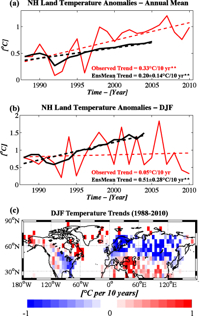
Figure 1. (a) The annual-mean area-averaged land temperature anomalies (°C; averaged poleward of 20°N) from 1988–2010 from CRUTEM3 (solid red) and the ensemble mean temperature anomaly from the historical scenario of the CMIP5 models (solid black). Also shown is the linear trend for the observations (dashed red) and the CMIP5 ensemble mean (dashed black), including ±1 standard deviation. A double asterisk (**) indicates trends significant at the p < 0.01 level. (b) As in (a) but for DJF-averaged observed temperature anomalies (red) and the CMIP5 ensemble mean DJF temperature anomalies (black). (c) The spatial pattern of linear trends in DJF surface temperature (°C/10 yr) from CRUTEM3. In (a) and (b), the plots of model-based anomalies are shifted vertically so that the anomaly in 1988 matches that from the observations.
Download figure:
Standard imageOur argument for how a warming trend globally can yield colder NH extratropical winters is summarized in figure 2. The July, August and September (JAS) surface temperature trend averaged over the Arctic (60–90°N) illustrates strong warming (figure 2(a)), which continues through the autumn (see supplementary figure S2 for the temperature trends for all four seasons, available at stacks.iop.org/ERL/7/014007/mmedia). Strong high-latitude warming during the late summer and early autumn enhances Arctic sea ice melt, as seen with the strongly negative trends in sea ice coverage (figure 2(b)), though the interaction is not one way as less sea ice also contributes to warmer Arctic temperatures. The combination of enhanced latent heat flux over the open waters of the Arctic and the effect of the Clausius–Clapeyron relationship increases lower tropospheric moisture over the Arctic. Indeed, this is what is observed in both MERRA (figure 2(c)) and radiosonde data (Durre et al 2009, figure 3). Recent studies have also linked decreasing sea ice with increased autumn cloud cover over the Arctic and an increase in precipitating clouds over Siberia (Eastman and Warren 2010, Stroeve et al 2011). Furthermore the modelling studies of Ghatak et al (2010) and Orsolini et al (2011) illustrate that decreasing Arctic sea ice can produce increased snowfall over Siberia. How much of the moisture increase is due to increases in temperature alone versus increased latent heat fluxes from increasingly open Arctic Ocean requires further investigation.
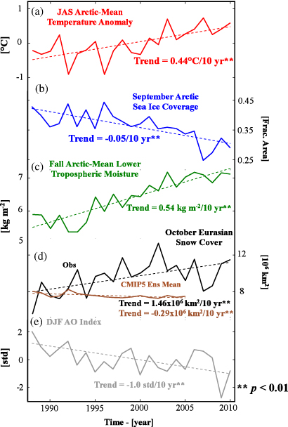
Figure 2. (a) JAS area-averaged (poleward of 60°N) surface temperature anomalies (°C) from NASA MERRA. (b) September area-averaged (poleward of 65°N) Arctic Ocean sea ice coverage (fractional area). (c) September–October vertically integrated (700–1000 hPa) and area-averaged (poleward of 60°N) specific humidity (kg m−2). (d) October mean snow cover areal extent (106 km2) over the Eurasian continent from observations (black) and the ensemble mean from the historical runs of the CMIP5 model output (brown line). (e) The DJF average AO index (standardized). Same-coloured dashed lines in (a)–(e) represent the linear trend in each index. A double asterisk (**) indicates trends that are significant at the p < 0.01 level.
Download figure:
Standard image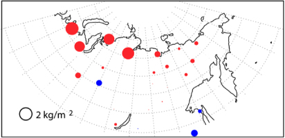
Figure 3. Change in October precipitable water (kg m−2) from various radiosonde stations based on the linear trend calculated over the period 1990–2010. The circle bottom left in the plot is shown for scale. Red circles indicate a positive trend and blue circles indicate a negative trend.
Download figure:
Standard imageAn increase in available moisture potentially results in higher precipitation efficiency over Siberia, where temperatures are still sufficiently cold enough to yield snow, which is consistent with the studies of Ghatak et al (2010) and Orsolini et al (2011). Figure 2(d) illustrates that the mean October snow coverage over the Eurasian continent has increased over the last two decades (figure 2(d); black curve), contrary to the expected negative trend predicted by the coupled models (figure 2(d); brown curve). So, there is an unexpected asymmetric trend not only in seasonal temperatures but also in Siberian snow cover, with increasing continental autumn snow cover amidst an observed hemispherically shrinking cryosphere (Solomon et al 2007, Flanner et al 2011).
Increasing autumn snow cover has important dynamic implications for the winter climate as its variability can force the wintertime phase of the AO, the leading mode of wintertime climate variability in the NH (Gong et al 2002, Fletcher et al 2007, Orsolini and Kvamsto 2009, Allen and Zender 2010, 2011). As discussed in Cohen et al (2007), increasing snow cover leads to stronger diabatic cooling and a strengthened Siberian high. This further leads to an increase in upward propagation of planetary waves, a weakened polar vortex and westerlies, but strengthened meridional flow. This results in a negative AO in the lower troposphere and increased Arctic outbreaks into the middle latitudes. The increasing trend in Eurasian snow cover over the past two and a half decades is concomitant with an overall weakening of the polar vortex (Alexeev et al 2011) and, as seen in figure 2(e), a negative trend of the AO. The negative AO trend favours anomalously cold temperatures over the eastern United States and northern Eurasia and increased storminess in the middle latitudes (Thompson and Wallace 1998, 2001).
Thus, the regional NH wintertime temperature cooling is directly tied to the declining trend in the wintertime AO, which is forced partly by increases in Eurasian snow cover during the autumn, driven in response to warmer surface temperatures at high latitudes prior to and concurrent with the autumnal advance in snow cover. While the AO certainly exhibits intrinsic behaviour, earlier studies predicted that global warming would be associated with a positive trend in the AO (as discussed in Cohen and Barlow 2005). Additionally, the negative trend in the AO has also been tied to decreasing Arctic sea ice (Honda et al 2009, Overland and Wang 2010, Petoukhov and Semenov 2010), aside from impacts of Eurasian snow cover variability. However, regressions of DJF surface temperature anomalies onto the winter AO, the October Eurasian snow cover, and the September Arctic sea ice coverage indices show stronger similarities between the snow cover and the AO pattern of variability than with the sea ice and AO variability (figure 4). Therefore, observational analysis suggests a first-order link between snow cover and the winter AO, with potential contributions to snow cover variability from sea ice variability and its effects on tropospheric moisture.
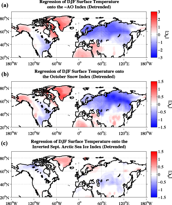
Figure 4. (a) Regression of DJF land surface temperature anomalies (°C) from NCEP/NCAR reanalysis onto the standardized inverted DJF AO index. (b) As in (a) but for regression onto the standardized October Eurasian snow cover index. (c) As in (a) but for regression onto the standardized inverted September Arctic sea ice index.
Download figure:
Standard imageThough the AO is a leading mode of high-latitude climate variability, other climate modes and forcings are important drivers of the extratropical circulation. To estimate the impact of modes other than the AO on the recent wintertime temperature trend, we computed the component of the temperature trend linearly related to the following large-scale climate modes and removed it from the overall trend: the El Niño/Southern Oscillation (characterized by the Niño 3.4 index), the Pacific Decadal Oscillation, the Atlantic Multidecadal Oscillation and sunspot number (figure 5). Only the AO explains a large fraction of the observed winter cooling trend; the direct impacts of other climate modes are negligible.
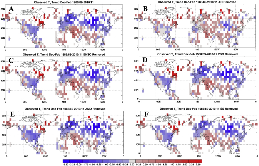
Figure 5. (a) The linear trend (°C/10 yr) in DJF land surface temperatures from 1988/89 through 2010/11. (b) As in (a) except the trend in the residual temperature anomalies after linearly removing the AO index. (c) As in (b) but linearly removing the Niño 3.4 index. (d) As in (b) but linearly removing the Pacific Decadal Oscillation index. (e) As in (b) but linearly removing the Atlantic Multidecadal Oscillation index. (f) As in (b) but linearly removing the influence of sunspot number. Values between − 0.25 and 0.25 are shown in grey, and missing and ocean values are shown in white. (a) and (b) are similar to figures 3(a) and (b) in (Cohen et al 2009).
Download figure:
Standard imageFinally, one rigorous test of our hypothesis is to use it in repeated successful predictions. Snow cover extent is used operationally to produce forecasts of winter surface temperatures, and these forecasts have produced highly skilful forecasts that were superior to forecasts that did not consider observed snow cover (Cohen and Fletcher 2007). This was true for the winter of 2009/10 (Cohen et al 2010) but especially for the winter of 2010/11 (figure 6), which was unique among seasonal forecasts in predicting a cold winter (Philadelphia Inquirer, 'Frigid Philadelphia-area weather expected to continue awhile', 9 January 2011). The pattern correlation between the observed and predicted temperature anomalies is 0.84. To further demonstrate the robustness of snow cover variability as a predictor, in figure 6(c) we also present the anomaly correlation coefficient for cross-validated hindcasts of surface temperature anomalies (1973–2010) only using October Siberian snow cover as a predictor. Such successful forecasts and robust hindcasts strongly support the argument that increasing snow cover has negated the background-warming signal and yielded a neutral boreal winter temperature trend for the last two decades or more.
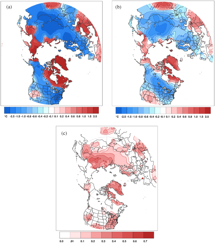
Figure 6. The (a) observed and (b) predicted winter surface temperature anomalies (°C) for the NH for December 2010–February 2011. The forecast for winter surface temperature anomalies in the seasonal forecast model relies on three main predictors: October Siberian snow cover, the October sea level pressure anomaly across northern Eurasia (a measure of the strength of the Siberian High), and the predicted winter state and phase of the El Niño/Southern Oscillation (i.e., the Niño 3.4 index). (c) The anomaly correlation coefficient for cross-validated hindcasts of land surface temperatures using Eurasian October snow cover extent as a predictor for winters 1973–2010. Only positive values are shown.
Download figure:
Standard imageIn summary, large-scale cooling has occurred during boreal winter over much of the NH landmasses over the last two and a half decades (figure 1(c)). With much attention on the effects of global warming on the climate system, the recent severe winter weather has heightened global warming scepticism among the general public. Traditional radiative GHG theory and coupled climate models forced by increasing GHGs alone cannot account for this seasonal asymmetry. Though we cannot conclude definitively that warming in the summer and autumn is forcing winter regional cooling, analysis of the most recent observational and modelling data supports links between strong regional cooling trends in the winter and warming trends in the prior seasons. A warmer, more moisture-laden Arctic atmosphere in the autumn contributes to an increase in Eurasian snow cover during that season. This change in snow cover dynamically forces negative AO conditions the following winter. We deduce that one main reason for models failing to capture the observed wintertime cooling is probably their poor representation of snow cover variability and the associated dynamical relationships with atmospheric circulation trends (Hardiman et al 2008, Jeong et al 2011). Incorporation of the snow cover–AO relationship into seasonal forecasts is shown to greatly improve their abilities, and hence long-term climate solutions from coupled climate models may also benefit from improved snow–AO relationships.
Acknowledgments
JLC is supported by the National Science Foundation (NSF) grants ARC-0909459 and ARC-0909457, and NOAA grant NA10OAR4310163. MAB was supported by NSF grant ARC 0909272. VA and JEC were supported by the NSF grants ARC 0909525 and Japan Agency for Marine–Earth Science and Technology. The authors acknowledge the climate modelling groups listed in table 2 of this letter, the World Climate Research Programme (WCRP) Working Group on Coupled Modelling (WGCM), and the Global Organization for Earth System Science Portals (GO-ESSP) for producing and making the CMIP5 model simulations available for analysis.