

Abstract
As a result of uncertain resource availability and growing populations, city managers are implementing conservation plans that aim to provide services for people while reducing household resource use. For example, in the US, municipalities are incentivizing homeowners to replace their water-intensive turfgrass lawns with water-efficient landscapes consisting of interspersed drought-tolerant shrubs and trees with rock or mulch groundcover (e.g. xeriscapes, rain gardens, water-wise landscapes). While these strategies are likely to reduce water demand, the consequences for other ecosystem services are unclear. Previous studies in controlled, experimental landscapes have shown that conversion from turfgrass to shrubs may lead to high rates of nutrient leaching from soils. However, little is known about the long-term biogeochemical consequences of this increasingly common land cover change across diverse homeowner management practices. We explored the fate of soil nitrogen (N) across a chronosequence of land cover change from turfgrass to water-efficient landscapes in privately owned yards in metropolitan Phoenix, Arizona, in the arid US Southwest. Soil nitrate ( –N) pools were four times larger in water-efficient landscapes (25 ± 4 kg
  –N/ha; 0–45 cm depth) compared to turfgrass lawns (6 ± 7 kg
  –N/ha). Soil
  –N also varied significantly with time since landscape conversion; the largest pools occurred at 9–13 years after turfgrass removal and declined to levels comparable to turfgrass thereafter. Variation in soil
  –N with landscape age was strongly influenced by management practices related to soil water availability, including shrub cover, sub-surface plastic sheeting, and irrigation frequency. Our findings show that transitioning from turfgrass to water-efficient residential landscaping can lead to an accumulation of
  –N that may be lost from the plant rooting zone over time following irrigation or rainfall. These results have implications for best management practices to optimize the benefits of water-conserving landscapes while protecting water quality.
Export citation and abstract BibTeX RIS
1. Introduction
Water conservation is a critical sustainability goal in urban areas worldwide (Natural Defense Resource Council (NDRC) 2008, Hilaire 2009, NOAA 2014). Weather extremes, increasing urban sprawl and population density, and the additive effects of urban heat islands create challenges in urban water management for even the most water-secure cities (Morehouse 2000, Vörösmarty et al 2010, Jenerette et al 2013, Hogue and Pincetl 2015). Since the late 1960's, water conservation programs have been developed to reduce residential water use (Gleick 2014). Because approximately 30%–50% of household water is consumed outdoors for landscaping (Domene and Saurí 2006, US Environmental Protection Agency 2015), conservation programs that target outdoor irrigation are key to reducing urban water consumption (Balling et al 2008, Ontario Water Works Association (OWWA) 2008).
Common conservation programs in cities incentivize the replacement of water-intensive turfgrass lawns with water-efficient landscapes that typically consist of interspersed drought-tolerant shrubs and trees with rock or mulch groundcover (e.g. xeriscapes, green infrastructure, rain gardens, climate-appropriate/water-wise landscapes, and others). In 2015, 77 cities in 16 US states offered financial incentives to encourage homeowners to replace their lawns. This land cover change from turfgrass to mixed shrubs and trees reduces water and often fertilizer use (Sovocool et al 2006, Hilaire 2009) but may have unintended consequences for water quality (Amador et al 2007). In non-urban ecosystems, the change from grassland to shrubland leads to loss of nitrogen (N) from the plant-soil system through erosion, runoff, and leaching (Parsons et al 1996, Turnbull et al 2010, Yusuf et al 2015). These losses are due to reduced soil-stabilizing roots, increased surface water runoff, changes in soil moisture (SM), and inconsistent plant nutrient uptake. Construction of shrub landscapes from fertile, managed urban grasslands may lead to similar water quality trade-offs, which could compromise water resource sustainability objectives.
While cities expand, turfgrass cover continues to be the land cover of choice for homeowners and businesses (Gaston et al 2005, Zhang et al 2015). Cultivated turfgrass covers more US land area (163 800 km2) than the major irrigated crops combined, including corn (43 000 km2; Milesi et al 2005). Grassy lawns provide aesthetic benefits (Larson et al 2015), sequester high amounts of C, 14.4 kg m−2 compared to 8 kg m−2 in forests (Pouyat et al 2006), and mitigate the urban heat island effect through evaporative cooling (Jenerette et al 2011, Hall et al 2015). However, lawns require substantial water inputs (on average 1 liter/m2 daily) and consume 7–10 times more water in semi-arid climates compared to mesic regions (USDA, National Agricultural Statistics Service (NASS) 2003, Milesi et al 2005, USDA, National Institute of Food and Agriculture (NIFA) 2011). As an alternative, shrub-dominated landscapes are promoted for their water savings (35%–75% reduction compared to turfgrass) in addition to aesthetic and biodiversity benefits (McPherson 1990, Sovocool et al 2006, Beumer and Martens 2015, and others).
As urban land cover increases, the ubiquity of intensively managed turfgrass has led to concerns about water pollution due to surface runoff and nutrient leaching (Petrovic 1990, Kasper et al 2015). Urban grasslands can contain as much N as agricultural soils due to intensive nutrient inputs, held mostly within a dense network of actively growing roots (Baer et al 2002, Raciti et al 2008, Reuben and Sorensen 2014). Nitrogen compounds such as nitrate  are highly mobile in the soil and contribute to contamination and eutrophication of ground water and aquatic ecosystems (Paul and Clark 1989). Some studies have shown that N losses from leaching and runoff can be high from lawns (Easton and Petrovic 2004, Raciti et al 2011, Wherley et al 2015 and others), however, recent research shows that turfgrass lawns retain more nutrients than previously thought, maintaining small pools of soil N and supporting surprisingly low rates of
  –N leaching (Martin 2001, Zhu et al 2006, Groffman et al 2009, Martinez et al 2014). In Baltimore, MD, Raciti et al (2008) found that turfgrass had higher N retention rates up to one year after 15N addition compared to forest plots. This pattern was likely due to accumulation of soil organic matter (McClellan et al 2009) and high plant uptake/productivity (Nektarios et al 2014), as well as N immobilization (Raciti et al 2008).
Much less is known about the fate of soil nutrients in water-conserving landscapes, particularly relative to the turfgrass lawns these landscapes replace. One study in artificial plots concluded that shrubs are more effective at using water and nutrients than turfgrass (Qin et al 2013). However, other studies in experimental landscapes show that gardens with wood mulch and shrubs have the potential to lose up to 10-fold more N than grass landscapes (Erickson et al 2001, Amador et al 2007, Loper et al 2013). After turfgrass death, rates of  –N leaching are high due to diminished plant uptake and changes in microbial activity (Jiang et al 2000, Hull et al 2001). In arid and semi-arid climates
  –N leaching can be exacerbated after precipitation due to accumulation of soil nutrients during long dry periods in shrubland ecosystems (Austin et al 2004, Vourlitis and Fernandez 2015). Thus, conversion of turfgrass to managed shrub landscapes may alter rates of biogeochemical cycling, with possible unintended consequences for aquatic resources.
Despite the growing prevalence of climate-appropriate landscapes, no studies to date have characterized the biogeochemical outcomes of this land cover change in heterogeneous residential areas. In this study, we explore soil properties and nutrient cycling across a chronosequence of land cover change from managed urban grassland to shrubland in yards of single-family homes in metropolitan Phoenix, Arizona, in the US Southwest. We hypothesized that the replacement of turfgrass with water-efficient landscapes would initially create disturbed, moist soils that would favor mineralization of organic N, nitrification, and mobilization of  –N due to limited and heterogeneous N uptake by shrubs. Furthermore, we hypothesized that soil nutrient content would decrease with water-efficient yard age (time since land cover change) as water inputs cause downward movement of nutrients in the soil, or as nutrients are taken up by maturing vegetation. Because homeowners and landscapers determine vegetative structure, composition, and maintenance of yards, we hypothesized that soil N in water-efficient landscapes would vary with differences in homeowner management. Elucidation of the patterns and drivers of residential landscape nutrient dynamics will help shape best management practices to achieve multiple sustainability outcomes in urban and suburban areas.
2. Experimental design and methods
2.1. Site selection
We explored the soil biogeochemical outcomes of a residential land cover change in the City of Tempe, Arizona (USA), a city of 168 000 residents within metropolitan Phoenix (United States Census Bureau 2014). Tempe is located in the Sonoran Desert, within the Central Arizona–Phoenix Long Term Ecological Research site (CAP LTER). The climate is arid, with annual precipitation at 18.3 cm split approximately evenly between two rainy seasons, summer monsoon and winter rains (Guido 2008, Maricopa County, AZ 2015). All residential sites in this study (referred to as 'yards') have been residential for at least 40 yrs. This long land cover history was chosen because the length of time in residential use significantly alters the soil nutrient content (Lewis et al 2006). Soils within each landscape class (turfgrass and all ages of water-efficient landscapes) are stratified across three soil series and two soil orders, Avondale clay loam (Typic Torrifluvents), Laveen clay loam (Typic Haplocalcids), and Contine clay loam (Vertic Calciargids) (appendix
2.2. Sampling design
We sampled front yards of homes that were landscaped with either turfgrass or desert-style, water-efficient yards during the summer monsoon season (between May and August of 2014). Forty-one water-efficient landscapes were selected using a homeowner survey, all of whom received financial incentive for turfgrass removal between 1993 and 2014 via the Tempe Landscape Rebate Program. Using convenience sampling, we also selected six single-family homes with turfgrass lawns that varied by irrigation type (flood, sprinkler) and tree cover. We grouped the participating households (n = 47) into five age categories (n = 5–8 per category): <4, 4–8, 8–13, and 18–21 yrs since land cover change, and turfgrass yards (figure 1). Water-efficient yards varied greatly in their area, structure, and vegetative composition as well as management (table 1, appendix
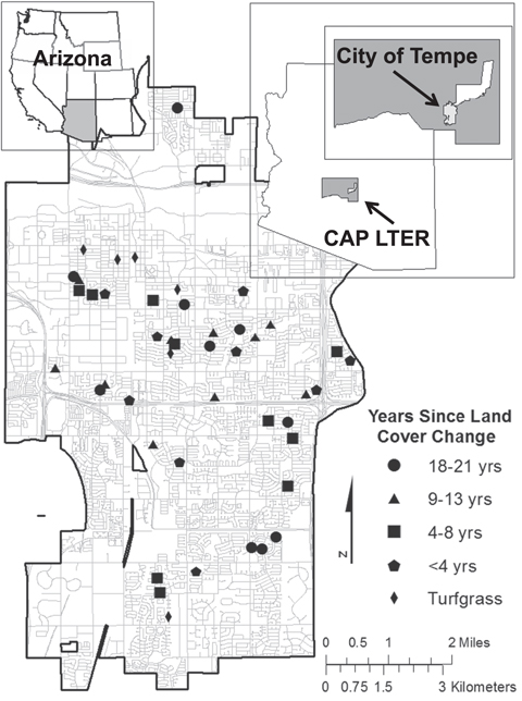
Figure 1. Map of Tempe, AZ within the CAP LTER study area, in the state of Arizona within the western US. Study yards are indicated by year since land cover change from turfgrass to water-efficient yards (n = 5–8 houses per category). All yards are located in areas that have an agricultural history but have been under urban land cover for >40 years.
Download figure:
Standard image High-resolution imageTable 1. Yard characteristics, divided by categories of years since land cover change. Yard area includes the front of house from the sidewalk or property edge to the house overhang and includes both pervious and impervious surfaces (e.g. driveway and walkway). Values represent the mean (±standard error [SE]). P-values are results of ANOVA tests between age categories within columns. Lowercase letters represent significant differences in shrub cover between age categories.
| Canopy cover | ||||
|---|---|---|---|---|
| Years since land cover change | Shrubs | Trees | N-fixing trees | Yard area |
| Years | % | % | % | m2 |
| Turfgrass | 11.73 (4.68) ab | 60.24 (8.29) | 18.00 (13.35) | 290.25 (67.59) |
| <4 | 17.08 (3.50) ab | 43.71 (6.66) | 26.02 (9.15) | 196.87 (15.05) |
| 4–8 | 17.66 (2.45) a | 57.03 (17.68) | 25.05 (9.33) | 255.97 (33.22) |
| 9–13 | 8.21 (1.92) b | 56.90 (10.87) | 27.78 (11.66) | 205.16 (22.33) |
| 18–21 | 15.09 (1.90) a | 57.92 (9.57) | 42.10 (9.96) | 185.69 (11.56) |
| F-value | 4.31 | 0.21 | 1.11 | 3.45 |
| p-value | 0.004** | 0.65 | 0.36 | 0.07 |
Note: **Shows statistical significance at p < 0.01.
2.3. Yard vegetation
We quantified the area of ground cover, and percent canopy cover of shrubs (plants shorter than 1.5 m, including cacti and perennial plants) and trees in the front yards of homes (from sidewalk to house overhang) using visual surveys. We also recorded the percent of the yard area covered by the canopies of trees with N-fixing associations. Vegetation cover observations were calibrated among researchers on five sample study yards to ensure consistency of data collection (±5%).
2.4. Soil sampling
To explore soil properties, we collected soil samples in June and July of 2014, the seasonal dry period prior to the summer monsoon. In each yard, we used a slide-hammer corer to collect four, 5 cm diameter cores split into three 15 cm depth intervals to 45 cm. We took two of the four cores under randomly chosen shrubs <1.5 m in height, excluding cacti (referred to as 'under plant') and the remaining two cores from adjacent vegetation-free patches between shrubs (referred to as 'between plant'). We sampled the homogeneous lawn area of turfgrass yards by taking only two soil cores in these sites (split into three depth categories). Prior to analysis, we homogenized the 2 cores within each patch type (under plants, between plants, turfgrass) and depth category in each yard (n = 6 samples in water-efficient yards; n = 3 samples in turfgrass yard). (For supplemental soil methods see appendix
2.5. Ion-exchange resin bags
We measured N availability in soils using buried ion-exchange resin bags (mixed Dowex Marathon MR-3) during the summer (July–September) and winter (December–February) rainy seasons to capture nutrient movement during precipitation events (Giblin et al 1994). We placed four resin bags in each yard at two depths, 5 and 30 cm, adjacent to the soils cores taken in the 'under plant' and 'between plant' patch types (appendix
2.6. Rainfall
The precipitation during each resin bag deployment was summed for each house, using precipitation data from the nearest tipping bucket rain gauge within the Flood Control District of Maricopa County sensor network (Maricopa County 2015).
2.7. Soil analyses
We processed soil cores to explore patterns of nutrient pools and rates of microbially mediated N transformation (extractable  –N and ammonium [
 –N] content, potential net N mineralization, potential net ammonification, and potential net nitrification) and soil properties related to N cycling (gravimetric moisture (SM), water-holding capacity (WHC), organic matter content (OM), and texture). All soil methods were based on LTER standard protocols (Robertson et al 1999).
We quantified pools of soil exchangeable  –N and
  –N by extracting soils in 2 M KCl within 48 h of collection to retain field conditions. To measure microbial N processes, soils were extracted after a 7 day incubation at 24 °C in the dark for 7 days at 60% WHC, optimal for aridland microbial communities (Sponseller 2007). We used a colorimetric phenolate method to measure
  –N +
–N + –N [reported as
  –N] and colorimetric cadmium reduction to measure
  –N concentrations in soil extracts (Lachat Instruments, Loveland, Colorado). Inorganic N values were amended with soil bulk density (BD) to determine pools from concentrations (Lee et al 2009, See appendix
Soil texture was determined using the hydrometer method (appendix
2.8. Statistical methods
We used mixed model analyses of variance to assess the relationship between the independent variables of landscape type (turfgrass and water-efficient) and year since land cover change (k = 4 categories; also referred to as 'landscape age') on the dependent variables of soil  –N (referred to as 'extractable
  SM, soil OM, and soil texture with site as a random factor. To assess patterns of resin
  –N (referred to as 'plant-available
  Binkley 1984) and
  –N availability, we used an Analysis of Covariance (ANCOVA) with precipitation as a covariate. When comparing whole yard averages (across depth and patch type) we weighted response variables by patch type as assessed by percent shrub cover in each yard (table 1). To evaluate how multiple management factors (independent variables: shrub cover, patch type, irrigation frequency, presence of plastic, and depth) influence water-efficient
  –N pools, we also performed a mixed linear model with yard as a random factor, using REML/GLS methods (Hrong-Tai and Cornelius 1996). Modified backward stepwise removal was used to create a model of water-efficient extractable
  –N levels by including only significant factors and ecologically relevant interactions, while avoiding Type I error (Mundry and Nunn 2009). We left all main effects in the model if they were significant or had a significant higher-order interaction (see appendix
3. Results
3.1. Soil nitrate content and availability differ by landscape type and across time
Conversion of residential 'grassland' to 'shrubland' significantly alters the availability and pool size of soil  –N, and varies across landscape age (figure 2). Using patch-weighted averages, water-efficient yards contained 25 ± 4 kg
  –N/ha in the first 45 cm of soil, while lawns contained much less, at 6 ± 7 kg
  –N/ha. Pools of soil extractable
  –N were relatively small and did not differ between yard type (mean 1.5 kg
  –N/ha). Soil extractable
  –N differed significantly by age category depending on patch type, where the decline in
  –N in the oldest landscapes was greatest in the patches between plants (Patch type x year since land cover change interaction, p = 0.01, table 2)1
.
–N in the oldest landscapes was greatest in the patches between plants (Patch type x year since land cover change interaction, p = 0.01, table 2)1
.

Figure 2. Pools of soil extractable  –N increase after a change from turfgrass to water-efficient landscapes (0–45 cm). Bars represent means of extractable
  –N by years since land cover change as a function of patch type. Error bars show ± one SE (n = 5–8 in each land cover category).
Download figure:
Standard image High-resolution imageTable 2. Values represent mean soil properties averaged over soil depth (0–45 cm), data split by soil depth in supplementary materials). Bold values indicate whole-yard averages (patch-weighted in water-efficient yards). P-values indicate differences between categories of landscape type (turfgrass versus water-efficient landscapes) and years since land cover change (water-efficient yard 'year categories', k = 4) on patch-weighted data. One SE shown in parentheses.
| Gravimetric soil moisture | Water holding capacity | Soil organic matter | Extractable NO3-–N | Extractable NH4+–N | Sand | Silt | Clay | Soil C:N | Total C | Total N | Bulk density | |
|---|---|---|---|---|---|---|---|---|---|---|---|---|
| % | g H2O/g soil | % | kg ha−1 | kg ha−1 | % | % | % | % | % | g cm−2 | ||
| Turfgrass yard | 17.45 (2.50) | 0.63 (0.05) | 5.63 (1.13) | 5.7 (2.50) | 1.50 (0.56) | 39.71 (3.83) | 42.97 (1.96) | 17.32 (2.48) | 23.50 (2.98) | 1.78 (0.24) | 0.10 (0.01) | 0.96 (0.03) |
| Water-efficient yard <4 yrs | 9.70 (2.50) | 0.55 (0.05) | 4.78 (0.69) | 31.0 (5.36) | 1.7 (0.26) | 39.07 (3.83) | 22.59 (4.32) | 8.59 (1.78) | 39.15 (8.84) | 1.43 (0.29) | 0.06 (0.02) | 1.06 (0.02) |
| Between plants | 9.89 (1.20) | 0.53 (0.03) | 3.99 (0.36) | 27.7 (8.57) | 1.60 (0.45) | 46.21 (3.46) | 39.02 (2.20) | 14.77 (1.47) | 25.12 (4.73) | 2.07 (0.12) | 0.11 (0.01) | 1.07 (0.02) |
| Under plants | 10.19 (0.88) | 0.55 (0.02) | 4.03 (0.41) | 21.2 (11.10) | 1.50 (0.32) | 45.56 (3.22) | 39.52 (1.74) | 14.92 (1.59) | 28.66 (4.22) | 2.02 (0.19) | 0.08 (0.01) | 0.98 (0.06) |
| Water-efficient yard 4–8 yrs | 9.57 (1.46) | 0.51 (0.05) | 3.67 (0.47) | 35.0 (10.26) | 1.60 (0.35) | 47.35 (4.78) | 16.10 (3.02) | 7.40 (1.52) | 19.15 (2.37) | 1.06 (0.19) | 0.06 (0.01) | 1.14 (0.06) |
| Between plants | 9.07 (1.34) | 0.47 (0.02) | 3.74 (0.37) | 31.1 (16.85) | 1.60 (0.34) | 48.10 (3.23) | 35.35 (1.66) | 16.55 (2.20) | 19.07 (2.06) | 1.59 (0.14) | 0.09 (0.01) | 1.04 (0.06) |
| Under plants | 9.22 (1.05) | 0.48 (0.01) | 3.67 (0.44) | 14.8 (6.61) | 1.20 (0.33) | 47.39 (2.59) | 36.84 (2.25) | 15.78 (1.93) | 22.42 (2.00) | 1.62 (0.13) | 0.08 (0.01) | 1.07 (0.04) |
| Water-efficient yard 9–13 yrs | 9.19 (1.10) | 0.48 (0.02) | 3.32 (0.30) | 35.0 (7.62) | 1.40 (0.24) | 46.55 (1.91) | 23.12 (4.10) | 8.75 (1.58) | 25.78 (3.05) | 0.83 (0.18) | 0.04 (0.01) | 1.40 (0.09) |
| Between plants | 9.27 (1.10) | 0.49 (0.02) | 3.34 (0.31) | 35.0 (11.64) | 1.40 (0.35) | 47.49 (2.21) | 38.09 (2.13) | 14.42 (0.97) | 21.13 (1.70) | 1.21 (0.10) | 0.06 (0.01) | 1.05 (0.05) |
| Under plants | 8.19 (0.47) | 0.50 (0.02) | 3.48 (0.32) | 34.8 (13.32) | 2.80 (0.80) | 45.59 (2.53) | 39.81 (2.69) | 14.60 (1.24) | 19.31 (2.17) | 1.40 (0.10) | 0.08 (0.01) | 1.06 (0.05) |
| Water-efficient yard 18–21 yrs | 9.10 (1.20) | 0.48 (0.02) | 2.92 (0.29) | 8.6 (1.13) | 1.40 (0.22) | 51.10 (2.20) | 17.40 (2.83) | 7.08 (1.35) | 35.67 (7.73) | 0.99 (0.18) | 0.03 (0.01) | 0.97 (0.05) |
| Between plants | 9.13 (1.27) | 0.47 (.02) | 2.80 (0.29) | 7.3 (2.14) | 1.40 (0.49) | 50.88 (2.34) | 34.86 (1.56) | 14.27 (1.49) | 57.49 (18.38) | 1.57 (0.14) | 0.05 (0.01) | 0.96 (0.06) |
| Under plants | 8.90 (1.35) | 0.49 (0.02) | 3.58 (0.41) | 16.5 (7.90) | 2.10 (0.78) | 51.19 (2.27) | 35.15 (1.59) | 13.66 (1.25) | 53.67 (15.41) | 1.85 (0.10) | 0.07 (0.01) | 1.03 (0.04) |
| F-value year category | 6.28 | 3.51 | 4.63 | 0.05 | 0.10 | 1.08 | 6.45 | 5.48 | 0.45 | 2.88 | 4.45 | 0.71 |
| p-value | <0.001*** | 0.02* | 0.004** | 0.82 | 0.75 | 0.40 | 0.01* | 0.02* | 0.51 | 0.05 | 0.01* | 0.41 |
| F-value landscape type | 25.72 | 9.56 | 8.17 | 4.27 | 0.04 | 6.56 | 15.43 | 12.96 | 0.22 | 6.09 | 7.91 | 2.65 |
| p-value | <0.0001*** | 0.003** | 0.007** | 0.04* | 0.84 | 0.01* | <0.001*** | <0.001*** | 0.65 | 0.023* | 0.01* | 0.11 |
Patch-weighted estimates of plant-available soil  –N and
  –N from resins did not differ between turfgrass (mean 0.32 mg
  –N/g resin and 0.04 mg
  –N/g resin) and water-efficient yards (patch-weighted mean 0.67 mg
  –N/g resin and 0.12 mg
  –N/g resin). Additionally, ANCOVA with summer precipitation revealed no relationship between years since land cover change or patch type. However, plant-available
  –N estimates were strongly and positively related to total precipitation (ANCOVA, p < 0.001, figure 3).
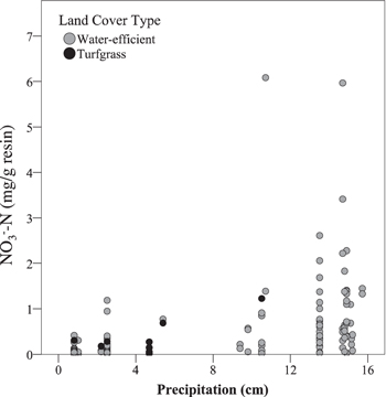
Figure 3. Plant-available  –N is significantly related to summer monsoonal precipitation received during the sampling interval. Data points represent mean plant-available
  –N over 4 months for each study yard. Precipitation values are sums of precipitation received (in cm) during the deployment period for each study yard.
Download figure:
Standard image High-resolution imageAs predicted, soil properties follow similar patterns to soil nutrients when turfgrass is replaced with a water-efficient landscape. Soil OM content was negatively related to soil  –N pools across patch types in water-efficient yards (Pearson's correlation p = 0.005, figure 4). Organic matter declined from 6% in turfgrass yards to 4% in water-efficient yards within 4 years after land cover change (ANOVA, landscape type x OM, p = 0.03), then declined further with time (ANOVA, year since land cover change x OM, p = 0.03). This pattern is confirmed by levels of total soil C and N which also decreased after land cover change (ANOVA, landscape type x C, p = 0.02 and landscape type x N p = 0.01). We found a proportional shift in the ratio of organic N to inorganic N between turfgrass and water-efficient yards, where turfgrass yard soils contained approximately 30% more organic N and 30% less inorganic N than the oldest water-efficient yards (table 2).

Figure 4. Soil organic matter (OM) content by year since land cover change, split by soil depth. Soil OM content declines over time. Error bars show ± one SE.
Download figure:
Standard image High-resolution imagePotential net N mineralization and net nitrification rates were not related to soil extractable  –N and did not differ between land cover types (appendix
3.2. Soil nitrate patterns influenced by management over time
Patterns in soil extractable  –N across landscape age were greatly influenced by yard management. Mixed linear model results between water-efficient yard extractable
  –N and yard biophysical and management variables identified several interactions that contributed significantly to the variation in soil
  –N in water-efficient landscapes of different age (table 3). The decline in soil
  –N over time was dependent upon patch type and was significantly related to the amount of irrigation, the presence or absence of plastic sheeting, and shrub cover. In yards that were converted >4 years prior to this study, landscapes irrigated more frequently (1+ times per week) contained less soil
  –N than yards that were not irrigated often (<1 time per week; p = 0.002). Soil
  –N did not differ by irrigation frequency in the youngest year category (figure 5). Shrub cover was also significantly and negatively related to extractable
  –N, and this pattern was strongest in the patches between plants (ANOVA, shrub cover x extractable
  –N, p = 0.01, shrub cover x location interaction, p < 0.01, figure 6).
Table 3.
Results of mixed model regression between soil extractable  –N and multiple management factors. Backward stepwise removal was used to create a model of water-efficient extractable
  –N levels by including only significant factors and ecologically relevant interactions. We left all main effects in the model if they were significant or had a significant higher-order interaction (appendix
| Factors and interactions | Df | F-value | p-value |
|---|---|---|---|
| (Intercept) | 180 | 5.49 | 0.02 |
| Years since land cover change | 41 | 0.27 | 0.61 |
| Shrub cover (%) | 41 | 9.87 | <0.01 |
| Patch type | 180 | 25.52 | <0.0001 |
| Irrigation frequency | 41 | 1.21 | 0.28 |
| Depth (cm) | 180 | 5.12 | 0.02 |
| Presence of plastic | 180 | 0.15 | 0.70 |
| Patch type:depth | 180 | 7.52 | <0.01 |
| Patch type:presence of plastic | 180 | 35.08 | <0.0001 |
| Years since land cover change:patch type | 180 | 13.30 | <0.001 |
| Shrub cover:patch type | 180 | 12.05 | <0.001 |
| Years since land cover change:irrigation frequency | 41 | 1.27 | 0.27 |
| Years since land cover change:patch type:irrigation frequency | 180 | 6.14 | 0.01 |

Figure 5. Frequent irrigation decreases soil  –N content in older yards compared to infrequent irrigation (0–45 cm). Values are averaged over soil depth and then weighted by patch type. Error bars represent ± one SE.
Download figure:
Standard image High-resolution image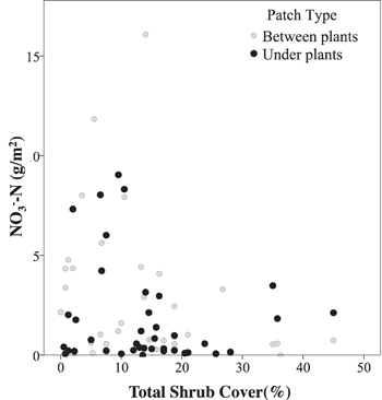
Figure 6. Shrub cover is inversely related to soil extractable  –N content.
Download figure:
Standard image High-resolution image4. Discussion
4.1. Mechanisms determining N availability after land cover change
Our study evaluated the fate of soil inorganic N in residential landscapes after homeowners converted their yards from water-intensive turfgrass lawns to water-efficient, shrub-dominated yards. Given the high rates of plant growth and soil organic matter turnover of turfgrass landscapes (Pouyat et al 2006), we hypothesized that the replacement of turfgrass with interspersed, drought-tolerant shrubs would lead to fast rates of decomposition that would in turn lead to excess inorganic N that would not be fully utilized by shrubs. Our results show that soil  –N pools, at 0–45 cm, increased in water-efficient yards, from below 2 kg N ha−1 in turfgrass soil to about 6 kg N ha−1 in water-efficient yard soil in the first 13 years after land cover change. This increase in plant-available N suggests that there is a pulse of soil organic matter decomposition and nitrification after turfgrass removal. In the first 5–8 years after land cover change, soil organic matter levels dropped from ∼6% to <4% while
  –N levels peaked, supporting the premise that elevated rates of organic matter decomposition and subsequent nitrification are a possible mechanism driving the production of plant-available N in water-efficient landscapes.
Interestingly, we found that soil  –N pools and total soil N declined in older water-efficient landscapes to levels comparable to turfgrass despite an increase in cover of N-fixing trees. These patterns could result from nutrient uptake by increasingly mature plants in older landscapes, or from N leaching to deeper soil layers after rain events (particularly in the patches between shrubs). Because available water is required for plant uptake in arid environments (Ogle and Reynolds 2004), and dry periods in the desert can lead to nutrient accumulation (Schlesinger et al 1996), balancing irrigation with plant needs is an important way to minimize potential leaching of N.
The shift in texture from silt loam to sandy loam after land cover change may result from tillage during the conversion process, removal of thatch and organic matter that provided structure to the upper soil-held silt content, and general disturbance of the topsoil during yard transformation and subsequent management. These textural changes, along with a decline in soil organic matter content, could augment rates of water infiltration, increasing nutrient mobility at depth (Austin et al 2004). Studies from experimental landscapes show that shrub installation replacing turfgrass leads to  –N leaching below the rooting zone (Amador et al 2007, Bushoven et al 2000). Our results show concentrations of
  –N in soil solution in water-efficient yards (0.4 mg to 1.4 mg
  –N/g resin) are not significantly higher compared to turfgrass yards at any depth (0.6 mg
  –N/g resin). This non-significant finding could be an artifact of the low precipitation received by turfgrass sites due to timing of resin deployments, which did not capture most of the larger monsoon events of the summer and therefore are not represented at higher precipitation levels. Furthermore, turfgrass soils contained similar
  –N in soil pore water to water-efficient landscapes despite the fact that they are irrigated with up to 3 times more water (Sovocool and Rosales 2001, Sovocool et al 2006).
We also found that soil C:N ratios are greater in older water-wise landscapes compared to recently converted landscapes and yards with turfgrass. One explanation of this pattern is that the water-efficient yards are leaching dissolved organic N over time (McLauchlan 2006, Wherley et al 2015), but it is more likely that this is an artifact of declining inorganic N pools due to downward movement of N or plant uptake, as discussed above. Alternatively, soil microorganisms could be immobilizing inorganic N in older water-efficient yards if inorganic N pools are limited. The magnitude of difference in C:N ratios between yard types could partly be attributed to addition of soil/fertilizer or disturbance during the conversion process.
4.2. Drivers of variation in soil N
In addition to patterns in soil N, our findings highlight significant differences in soil and ecosystem properties across the turfgrass to water-efficient landscape transition (table 1). Homeowners and hired landscapers determine how their yard is converted, including how much and where vegetation is planted and how the landscape is maintained, as well as decisions that determine the magnitude of plant nutrient uptake, such as the type of vegetation and water inputs (appendix  –N content and that the cover of shrubs may be more important than trees in these landscapes. Differences in vegetation by species or life form (e.g. shrubs versus trees or cacti) influence root structure and patterns of nutrient uptake. For example, plants in semi-arid shrub-dominated ecosystems allocate a large fraction of their fine root mass to shallow soil layers, and their activity is highly dependent on water availability (Schwinning and Sala 2004). If nutrient-acquiring roots are concentrated at shallow depths, they will have a diminished opportunity to intercept plant-available
  –N deeper in the soil profile (Schenk and Jackson 2002, Amador et al 2007). Plant root structure is also affected by water availability. Frequent irrigation with small amounts would encourage shallow root growth, while infrequent but large irrigation events may increase rates of water infiltration, leading to deeper rooting such that shrubs could access water several days after an irrigation event (Rundel and Nobel 1991).
5. Conclusions
This research is the first to explore the ecological outcomes and temporal dynamics of an increasingly common urban land cover that is universally promoted in US cities and growing in popularity worldwide. Increasingly common droughts, exacerbated by augmented rates of evaporation from warmer global temperatures, intensify the need for programs that aim to decrease urban water use (Sheffield et al 2012). Many cities already restrict the number of days water can be used for landscaping, and a subset of those cities incentivize homeowners and businesses to decrease water use (Environment Agency 2009, California, Department of Water Resources 2015, WaterSense, U.S. Environmental Protection Agency 2015). Often the restrictions on water use are local initiatives, starting at the municipal or even citizen level. As climate uncertainty continues and urban areas and population density increase (Kirtman et al 2013, World Health Organization 2015), it is likely that there will be progressively more top-down implementation of statewide or federal regulation of water use (Walton and Hume 2011, Clarvis and Engle 2015, Desert Water Agency 2015, Mass.gov. 2015). Severe droughts and over-allocation of the Colorado River Basin in the Western US have lead to recent legislation to decrease urban water use, such as California's mandate of 25% reductions by 2016 (Castle et al 2014, Department of Water Resources 2015). Water-wise alternative landscapes are already at the forefront of the initiatives being applied to accomplish water use reduction goals, and these landscapes will likely continue to gain popularity in urban areas.
Results from our study show that water availability and management are significantly associated with the amount and mobility of  –N in soil. For this reason, installment of water-efficient yards in more mesic climates—or soils with sandy textures as is common in coastal areas—could result in faster rates of organic N mineralization and increased concentrations of leached
  –N within a shorter time period than measured in this study (for example, see Erickson et al 2001). The likelihood of N leaching will depend on several factors, including soil type, total water inputs (irrigation frequency/amount and precipitation) and vegetation cover. However, our research suggests that installation of sparsely distributed shrubs would decrease yard N uptake capacity, especially within the first few years after landscaping. Furthermore, while irrigation frequency/amount is likely to be significantly lower in mature water-efficient yards, landscapes are frequently irrigated during shrub establishment (Erickson et al 2001). Additionally, the high SM we measured in water-efficient yards (∼10%) likely exceeds plant requirements, which corroborates other studies that suggest landscape over-watering is common (Volo et al 2015). In order to prevent the accumulation of available
  –N in lawn-alternative landscapes and mitigate the potential for negative water quality, we recommend that future research should develop best management practices and explore the outcomes of residential land cover change. For example, removing grass using a turf cutter could eliminate a large source of organic material in new landscapes; soil amendments, such as fertilizer or compost, could be added only where shrubs will be planted; and adding both annual and perennial ground cover may contribute to nutrient retention with minimal water input. Additionally, future research in water-efficient landscapes across gradients of precipitation and yard structure is necessary in order to determine potential trade-offs between water conservation and water quality.
Acknowledgments
We would like to thank all of our study participants in the City of Tempe; Kelli Larson and Diane Pataki for their guidance and feedback throughout this research; Richard Bond at the City of Tempe for connecting us with homeowners and providing insight into Tempe's rebate program; ASU's School of Life Sciences, the Graduate and Professional Student Association, and CAP LTER for proving financial support to make this research happen; and the technical assistance from Stevan Earl and Jennifer Learned. This material is based upon work supported by the National Science Foundation under grant number BCS-1026865, Central Arizona–Phoenix Long-Term Ecological Research (CAP LTER); and grant number EF-1065740, Macrosystems Biology.
Appendix A. Lab and field methods:
Appendix.
Study site. The city of tempe is located within the Phoenix metropolitan area, within the boundaries of the 6400 km2 Central Arizona–Phoenix Long Term Ecological Research site (CAP LTER). The climate is arid, with annual precipitation split between the summer monsoon (July to September), characterized by sporadic, short, and heavy rainfall, while winter brings longer but lighter rainfall events. Soils in the study area are Laveen loam/Laveen clay loam (Fine-loamy, mixed, superactive, calcareous, hyperthermic Typic Torrifluvents), Contine clay loam (Fine, mixed, superactive, hyperthermic Vertic Calciargids) or Avondale clay loam (Coarse-loamy, mixed, superactive, hyperthermic Typic Haplocalcids) derived from flood-plain parent material with a slope of 0%–1% (Soil Survey Staff 2013). All residential sites used in this study (referred to as 'yards') have been under urban land use for at least 40 yrs and have an agricultural land legacy (Knowles-Yanez et al 1999). Annual temperatures range from average high of 30 °C to average lows of 12 °C (NOAA 2015). In 1993, Tempe was one of the first cities in the nation to offer financial rebates to replace turfgrass lawns with drought-tolerant shrubs. Since then, the city has kept records of participants in the Tempe Landscape Rebate Program, documenting the address, homeowner name, as well as yard area and rebate year. Common yard plants in Tempe water-efficient yards include both native and non-native species of cacti, such as saguaro (Carnegiea gigantea), prickly pear (Genus Opuntia), and barrel cacti (Genus Echinocactus); shrubs, such as creosote (Larrea tridentata), brittlebush (Encelia farinose), and Mexican bird of paradise (Caesalpinia pulcherrima), among others, and N-fixing trees, such as mesquite (Prosopis chilenses and P. velutina), acacia (Acacia berlandieri and A. constricta), and palo verde trees (Parkinsonia florida and P. microphylla).
Appendix.
Household survey and site selection. We selected 1400 homes that participated in the Tempe Landscape Rebate Program, stratified by the year they received the rebate so that an equal number of homes were selected at random from each year. This rebate program offers a financial incentive to residents to encourage turfgrass removal and conducts voluntary classes on xeriscaping. In April of 2014, we sent postcards to the homes with a link to an online survey to gather data on yard history and management, and secure homeowner permissions for in situ research. We included survey questions that fell under three general categories: current yard cover and maintenance, the yard conversion process and motivations, and homeowner demographics. These categories provided information on how the homeowner managed his/her yard, as well as common practices used during the conversion process (table A1). We contacted individuals by post-card, written in English, which contained a link to the online survey. Homeowners were also given the option to participate in the survey over the phone or fill out a hard copy sent to their home.
Table A1. Selected survey questions and responses regarding yard management.
| Survey question topic | Survey question | % of yards |
|---|---|---|
| Conversion process | To the best of your knowledge, when your yard was changed to a desert-style landscape, how was the yard prepared? | |
| Stopped watering grass | 45.2 | |
| Living grass removed (removed grass while still alive) | 41.9 | |
| Stopped water and used herbicide | 38.7 | |
| Used turf removal equipment (removed first 5cm soil) | 22.6 | |
| Kept living grass (installed new cover over living grass) | 2.0 | |
| Other | 22.6 | |
| Soil amendments during conversion | Before adding rocks or other non-grass ground cover, which of the following activities were completed? | |
| Laid down barrier (plastic sheeting or weed-blocking fabric) | 22.6 | |
| Tilled soil | 16.1 | |
| Added soil or compost | 3.2 | |
| Watered grass or dirt | 0 | |
| Added fertilizer | 0 | |
| Other | 9.7 | |
| Litter management | Which of the following best describes what is done after maintaining the yard? | |
| Cut grass, weeds, leaves/branched and remove by bagging | 92.9 | |
| Leaf-blower is used to blow off leaves, weeds, or grass | 28.6 | |
| Grass clippings, leaves or weeds are left on the ground | 9.5 | |
| Grass, shrubs or weeds are not cut or trimmed | 2.4 | |
| Do not know | 2.4 | |
| Irrigation frequency | Thinking about this past summer (June–August 2013), about how often/were the plants, trees or grass in your yard usually watered? | |
| Every day | 4.8 | |
| Every week (but not daily) | 54.8 | |
| Every month (but not weekly) | 21.4 | |
| Every season (but not monthly) | 4.8 | |
| Never water | 11.9 | |
| Irrigation type | Please indicate all of the ways used to water plants, trees, or grass in your yard. | |
| Drip irrigation | 71.4 | |
| A handheld hose | 52.4 | |
| Watering jug/can | 35.7 | |
| Sprinklers | 31.0 | |
| Sprinklers on a hose | 14.3 | |
| Flood irrigation | 4.8 | |
| Other | 71 | |
| Decision making | Who makes decisions about how your yard is maintained? | |
| I do | 74.8 | |
| Another household member(s) | 19.2 | |
| Landscaping service | 2 | |
| Other | 4 | |
The response rate of the household surveys was 10% (n = 140) and of those, 40 individuals opted in for further study and their yards were used for soil sampling. All sites are single-family homes in the City of Tempe that have an agricultural land legacy. In order to avoid location bias we mapped the addresses using GIS software and visually assessed that the sites were spatially distributed across the city. We further grouped the participating households (n = 47) into age categories containing an approximately equal number of yards: <4, 4–8, 9–13, and 18–21 years since land cover change, and turfgrass yards (0 years since land cover change). This design provided multiple replicates for each category including grassy lawns as age zero (n = 5–8 per category).
Yard vegetation. Drought-tolerant shrubs, cacti, and desert-adapted trees are common in water-efficient yards in Tempe, but the number of plants and level of maturity is highly variable among the study sites. In order to identify potential effects of plant nutrient uptake on soil nutrient pools and fluxes, we quantified the area of ground cover, and canopies of shrubs and trees in the front yards of each home using visual surveys. For ground cover, we segmented yards into four quadrants and recorded the approximate cover of grass, gravel, bare soil, or impervious (pavement/stones), summing to 100% for each quadrant. The data for each quadrant were later multiplied by 0.25 and summed together to get a whole yard cover of each cover type. To determine canopy cover, we first measured the yard dimensions using a measuring tape to determine length, from the sidewalk (or street) to the front overhang of the house, and width, from one side of the lot to the beginning of the next lot, including impervious driveways or walkways. Length and width were multiplied to determine total yard area. We then measured the canopy cover of all trees (defined as vegetation taller than 1.5 m and excluding cacti) by taking two cross section measurements of each tree's canopy and multiplying these measurements to get a square area. To determine the percent yard canopy cover, we divided the total yard area by the total canopy of trees and then multiplied by 100. In order to capture any biogeochemical impacts from vegetation with N-fixing symbioses (or non-N fixing legumes with high tissue N content, such as palo verde trees), we also quantified canopy cover for these specific trees. Using the same method as the ground cover, we recorded the vegetative cover of non-trees (referred to as shrub cover, %) by visually segmenting the yard into four quadrants and assigning a % cover of shrubs for each quadrant. We defined shrubs as all plants that were shorter than 1.5 m, including cacti and non-annual plants.
Appendix.
Soil sampling. In turfgrass yards, we took four soil cores by choosing areas of the yard that were at least 1 m away from impervious surfaces and a 1 m away from any tree canopy. After homogenization by depth category and patch-type, samples were bagged and placed at 10 °C in a cooler with ice for 1–2 h until processing in the laboratory.
In the winter of 2014, we sampled soil to determine BD using a slide-hammer corer at 15 cm increments, down to 45 cm. The slide-hammer allowed us to penetrate to the desired depth in cemented soils (with a caliche layer). Most cores were extracted as whole cores with little impaction. Core holes were measured and compared to core length to test for impaction. We took special care to collect any soil that may have fallen back into the coring hole due to sandy or loose soils. Any site that had incomplete cores or visible impaction had an additional core taken. Samples were bagged and brought back to the laboratory for processing.
Appendix.
Ion-exchange resin bags. Resin bags were composed of nylon and filled with approximately 10 g of 50/50 cation/anion exchange resins (Dowex Marathon MR-3 hydrogen and hydroxide form). We placed four pairs of resin bags in each yard, two pairs each adjacent to but greater than 30 cm from the place where the 'between plant' and 'under plant' soil cores were taken. Resin bags were paired to control for small-scale spatial variation from nearby plants or large rocks. One of the pairs was placed at approximately 5 cm depth and a second pair was placed at approximately 30 cm. For the shallow pair, we used a shovel to lift the soil, then place the paired resin bags under the shovel and then removed the shovel to achieve the least amount of disturbance over the resin bag. To ensure soil sitting above the 30 cm resins was undisturbed and for easy removal and replacement at depth, we augured through the soil at an angle (30°–45°) to approximately 30 cm depth and inserted a PVC pipe that held the paired resins on one end (figure A1). Resins were kept in the yards for about two months, after which we replaced the resin bags with new resin bags in the same holes where they remained for another two-month deployment period.

Figure A1. The 30 cm depth resins were installed using a double-PVC pipe apparatus. The outside larger pipe was permanently installed at an angle in the soil during the study. The smaller, inner pipe, was used to hold and replace the resins. The resins sat at the bottom end of the tube (shown here upside down) and the opposite end was capped using plastic sheeting to prevent any precipitation or irrigation water reaching the resin bags that did not first travel through the soil column.
Download figure:
Standard image High-resolution image
After each two-month incubation period, we carefully removed the resin bags with a shovel and gloved hands to ensure all nutrients collected by the resins were from the soil. The resin bags were then placed in individual sealed plastic bags and put on ice at 10 °C in a cooler for 1–3 h until processing in the laboratory. If processing was postponed more than 3 h, resin bags were placed in the refrigerator up to 24 h. In the laboratory, we rinsed the resins with deionized water to remove any residual soil. We removed the nylon bag and then each pair of resin bags were homogenized and then dried for 48–72 h at 60 °C until they stopped losing weight. After drying, organic materials such as roots, were carefully removed using forceps. Resins were then extracted using 2 M sodium chloride (NaCl) solution by shaking for 24 h at 160 rpms. The supernatant was poured through pre-leached Whatman #1 filters and samples were frozen at −4 °C until further analyses up to 3 weeks after extraction.
Appendix.
Soil analyses. In the laboratory, we sieved the soils using a 2 mm sieve within 24 h of collection; gravel and organic matter (roots, leaves, insects) were discarded. 20 g of sieved soil was set aside at field moisture for both SM determination and WHC, and 10 g was weighed out for both exchangeable  and
and  analyses and for incubation to determine microbial N transformation rates. We air dried the remaining soil and stored it for future analyses. 20 g of soil was dried at 105 °C for 24 h, and then weighed to determine the moisture content. We determined WHC (100% field capacity of the soils) by saturating 20 g of loose soil in a WHC filter funnel using a Whatman #42 filter and weighing the soil after 24 h to determine water content. The 100% WHC value was multiplied by 0.6 to get the 60% WHC which provides soil microbes with both enough water and oxygen in soil pore spaces to optimize microbial processes on dry desert soils (Sponseller 2007). Optimizing microbial activity during the incubations allowed us to measure the greatest potential rates of microbial activity. To determine organic matter content, 10 g of oven-dried soils was combusted using a muffle furnace at 550 °C for 4 h and then weighed again to determine mass loss. We determined total soil C and total soil N using a CHN elemental combustion analyzer at the Goldwater Environmental Lab (PE 2400; Tempe, AZ).
To determine pools of soil exchangeable  and
and  we extracted the soils using 100 ml of 2 M potassium chloride (KCl) within 48 h of collection to retain field conditions. Soil extractions were shaken for one hr at 160 rpms and then we filtered the supernatant through pre-leached Whatman #1 filters. To measure microbial N processes, soils were incubated at room temperature (24 °C) and in the dark for 7 days at 60% WHC. After the incubation period, we extracted the samples in the same way as the initial soil nutrient samples using a 2 M KCl solution. After extraction all samples were frozen immediately and thawed when ready to analyze, within 4 weeks.
Appendix.
Soil texture. We determined soil particle size using the hydrometer method followed by sieving for sand (Day 1965). To disperse soil particles we shook 40 g of oven-dried soils with 100 ml of 50 g l−1 (5%) sodium hexametaphosphate for 24 h and then carefully transferred the soil to a sedimentation cylinder. We added 900 ml of deionized water to the cylinder and used a suspension plunger to manually suspend the soil in the cylinder. To determine sand (%) and silt (%) content, we took a hydrometer readings at 40 s and at 7 h respectively. We calculated clay content using the known percentage of sand and silt subtracted from 100%. To check accuracy of the 40 s sand readings, we sieved the soil after the 7 h reading using a 53-micron mesh size and determined sand weight by removing remaining sediment from the sieve and drying it overnight at 105 °C. The average organic matter content of all samples was 3.5%. According to Gasparotto et al (2003), not destroying soil organic matter prior to texture analyses decreases precision of silt content by only 1% when using the hydrometer method. Given the low organic matter content in our soils (average 3.5% of WE yards, 5.7% for turfgrass) the error in the silt values from not destroying the organic matter did not significantly affect the soil particle size distribution.
Appendix.
Bulk density. To estimate BD, we used a hybrid BD method recommended by Throop et al (2012) for rocky aridland soils, where BD = (mass of fine soil [<2 mm])/(core volume-volume of gravel [>2 mm]). Throop's review of BD methods suggests this correction for coarse volume is appropriate when using BD for nutrient analyses pertaining only to the fine fraction because the coarse fraction does not contain extractable inorganic N (table A2). Because volumetric BD estimates are inaccurate in rocky soils, we excluded cores in which the gravel volume was greater than 20%. We first calculated BD values for each soil sample then, because there was no significant difference between patch type, we averaged the BD for each yard across patch type within each depth category. We then averaged across yards, keeping unique BD values for each depth because of significant differences in BD between depth categories.
Table A2. Bulk density estimates (g m−3) for soil samples from 47 residential yards using three different methods (Throop et al 2012). Values are averages across patch-type because there was not a significant difference in BD between patch types. One standard error (SE) shown in parentheses.
| Estimates of bulk density using three methods. Coarse soil is >2 mm fraction and fine soil is <2 mm fraction. | |||
|---|---|---|---|
| Depth | Coarse + fine mass/core volume | Fine mass/core volume | Fine mass/(core volume–coarse volume) |
| cm | g cm−2 | ||
| 0–15 | 1.13 (.02) | 0.95 (.02) | 1.03 (.02) |
| 15–30 | 0.96 (.03) | 0.86 (.03) | 0.90 (.03) |
| 30–45 | 1.19 (.03) | 1.09 (.03) | 1.15 (.03) |
Appendix B. Microbial processes
Appendix.
Potential net N mineralization and net nitrification were both highly variable between years since land cover change categories as well as in the different patch-types (table B1). The only identifiable pattern is in the net N mineralization values, where mineralization was higher in the under plant patch-type than the between plant patch-type. Net ammonification was not as variable across year category and patch-type, however there was also no significant difference between the patch-weighted averages.erlaa301at6
Table B1. Soil microbial processes by year since land cover change and patch type. Bold rows are patch-weighted values. One SE in parenthesis.
| Net N mineralization | Net nitrification | Net ammonification | |
|---|---|---|---|
| μg N g−1 soil/day | μg N | ||
| Turfgrass | 0.32 (0.31) | −0.06 (0.02) | 0.38 (0.30) |
| Water-efficient yard <4 yrs | 0.28 (0.92) | 0.40 (0.91) | −0.12 (0.05) |
| Between plants | 1.04 (0.42) | −0.11 (0.04) | 1.15 (0.44) |
| Under plants | 1.44 (0.48) | −0.11 (0.04) | 1.54 (0.48) |
| Water-efficient yard 4–8 yrs | 1.12 (1.60) | 0.88 (1.74) | 0.24 (0.37) |
| Between plants | 0.71 (1.08) | 0.11 (0.15) | 0.60 (1.11) |
| Under plants | 1.11 (0.54) | 0.58 (0.37) | 0.53 (0.42) |
| Water-efficient yard 9–13 yrs | −0.12 (1.02) | −0.16 (1.01) | 0.03 (0.11) |
| Between plants | 0.10 (0.64) | −0.02 (0.05) | 0.12 (0.63) |
| Under plants | 1.14 (0.39) | 0.66 (0.46) | 0.48 (0.70) |
| Water-efficient yard 18–21yrs | 0.32 (0.09) | 0.43 (0.09) | −0.11 (.04) |
| Between plants | 0.26 (0.12) | −0.10 (0.03) | 0.37 (0.12) |
| Under plants | 0.81 (0.42) | −0.20 (0.05) | 1.01 (0.40) |
Appendix C. Results of mixed linear regression model selection
Appendix.
Table C1.
Results from mixed linear model selection using backward stepwise removal of independent variables (years since land cover change, shrub cover, patch type, irrigation frequency, presence of plastic, and depth) as they relate to soil extractable  –N in water-efficient yards. 'Years since' is the years since land cover change categories (<4, 4–8, 9–13, and 18–21). 'Shrub cover' is percent shrub cover. 'Irrigation frequency' is high or low frequency of irrigation (<1 time per week or 1+ times per week) 'Plastic present' is whether or not the yard had plastic sheeting down under the mulch layer.
| Model: All models include house as a random factor and use a restricted maximum likelihood criterion | AIC | AICc | dAICc | Weight [AICc] |
|---|---|---|---|---|
| NO3−–N∼Years since*Shrub cover*Patch type*Irrigation Frequency*Depth*Plastic Present | 472.60 | 525.56 | 750.54 | >0.000 |
| NO3−–N∼Years since+Shrub cover*Patch type*Irrigation Frequency*Depth*Plastic Present | 39.89 | 52.62 | 277.60 | >0.000 |
| NO3−–N-∼Years since+Shrub cover+Patch type*Irrigation Frequency*Depth*Plastic Present | −163.05 | −159.11 | 65.87 | >0.000 |
| NO3−–N-∼Years since+Shrub cover+Patch type+Irrigation Frequency*Depth*Plastic Present | −187.96 | −186.30 | 38.68 | >0.000 |
| NO3−–N-∼Years since+Shrub cover+Patch type+Irrigation Frequency+Depth*Plastic Present | −214.52 | −213.54 | 11.45 | 0.00 |
| NO3−–N-∼Years since+Shrub cover+Patch type+Irrigation Frequency+Depth+Plastic Present | −225.79 | −224.98 | 0.00 | 0.85 |
| NO3−–N-∼Years since+Shrub cover+Patch type+Irrigation Frequency+Depth+Plastic Present+ (Depth:Patch type)+(Location:Plastic Present)+(Years since:Patch type)+(Shrub cover:Patch type)+(Years since:Irrigation Frequency)+(Years since:Patch type:Irrigation Frequency) | −223.67 | −221.47 | 3.52 | 0.15 |
In order to identify the most important combination of variables in controlling soil N cycling in water-efficient landscapes, we used model selection, of a mixed linear model, with backward stepwise removal (table C1). Typical stepwise regression removes variables based only on their contribution to a 'best-fit' model, but this type of removal does not consider that some interactions and variables are important regardless of if they are found significant. For this reason, we performed a mixed linear model using backward stepwise removal to create a model that predicts water-efficient extractable  –N levels by including only significant factors and interactions that make sense ecologically. We left all main effects in the model if they were significant or had a significant higher order interaction. This table shows selection criterion for model possibilities. AICc was used due to low sample size. Model 6 had the lowest deltaAICc and highest weight, indicating that it is a model that explains the data well. We added ecological interactions that are important to
  –N levels to this simplified model, shown in model 7. Analyses were performed on transformed data.
Footnotes
- 1
Supplemental material online includes additional data and figures stacks.iop.org/ERL/11/084007/mmedia.