

Abstract
Despite documented intra-urban heterogeneity in the urban heat island (UHI) effect, little is known about spatial or temporal variability in plant response to the UHI. Using an automated temperature sensor network in conjunction with Landsat-derived remotely sensed estimates of start/end of the growing season, we investigate the impacts of the UHI on plant phenology in the city of Madison WI (USA) for the 2012–2014 growing seasons. Median urban growing season length (GSL) estimated from temperature sensors is ∼5 d longer than surrounding rural areas, and UHI impacts on GSL are relatively consistent from year-to-year. Parks within urban areas experience a subdued expression of GSL lengthening resulting from interactions between the UHI and a park cool island effect. Across all growing seasons, impervious cover in the area surrounding each temperature sensor explains >50% of observed variability in phenology. Comparisons between long-term estimates of annual mean phenological timing, derived from remote sensing, and temperature-based estimates of individual growing seasons show no relationship at the individual sensor level. The magnitude of disagreement between temperature-based and remotely sensed phenology is a function of impervious and grass cover surrounding the sensor, suggesting that realized GSL is controlled by both local land cover and micrometeorological conditions.
Export citation and abstract BibTeX RIS
1. Introduction
The urban heat island (UHI) effect is characterized by elevated temperatures in urban areas, relative to the surrounding countryside (Oke 1973, 1982, 1988). Though 60% of global population is expected to live in urban areas by the year 2030, the ecological impacts of the UHI remain poorly understood (Cohen 2006, Jochner and Menzel 2015). UHI-induced increases in temperature can affect plant phenology (the timing of developmental events such as leaf emergence and senescence) both within and around cities (Jochner et al 2012, Jochner and Menzel 2015). Understanding the UHI influence on phenology is critical, as the start of the growing season (SOS), end of the growing season (EOS), and total growing season length (GSL) can have substantial impacts on water, energy, and carbon exchange, which in turn have important feedbacks with climate (Penuelas et al 2009, Richardson et al 2013, Keenan et al 2014). UHI-induced changes in GSL have direct impacts on global food security, as 25%–30% of global urban residents, most commonly from the poorest sectors of the population, are involved in food production and 60% of irrigated agriculture (35% rainfed) is within 20 km of urban areas (Orsini et al 2013, Thebo et al 2014). Moreover, UHI-driven advances in spring may compound shifts in GSL that are already occurring due to climate change (Menzel and Fabian 1999, Schwartz and Reiter 2000) and thus increase the survival and activity of harmful insects and pathogens (Bradley and Altizer 2007).
Numerous observational studies have reported urban–rural phenological differences in Africa (Gazal et al 2008), Europe (Menzel and Fabian 1999, Roetzer et al 2000, Gazal et al 2008, Jochner et al 2012, Comber and Brunsdon 2015), Asia (Omoto and Aono 1990, Gazal et al 2008, Jeong et al 2011), and North America (Primack et al 2004, Gazal et al 2008, Neil et al 2010). These studies primarily select one or several species to monitor phenology at discrete points and are not designed to capture variability within urban areas (Mimet et al 2009, Fotiou et al 2011, Comber and Brunsdon 2015). While sensor networks are widely used to describe UHIs (see Schatz and Kucharik 2014 for a summary of previous work), very few studies have investigated the spatial variability of UHI effects on GSL (Todhunter 1996, Smoliak et al 2015).
Due to the difficulty in studying phenological variability from the ground, satellite remote sensing is often used to study spatial variability in GSL to understand the impacts and extent of the UHI. For example, White et al (2002), Zhang et al (2004), Fisher et al (2006), and Elmore et al (2012) found increases in GSL ranging from 0 to 15 d associated with urban areas in the eastern USA, with a zone of influence extending up to 32 km from the urban margin. However, each of these studies relies on either masking out urban areas to study exclusively deciduous forest in or near urban areas or uses satellite data so coarse in resolution that spatial heterogeneity is obscured. These limitations reduce our ability to explore drivers of GSL within urban areas, where the impacts of UHIs on phenology would likely be both strongest and most variable.
In this study, we combine a network of temperature sensors of near unprecedented density and extent (Schatz and Kucharik 2014, Smoliak et al 2015) with Landsat-derived phenological metrics at 30 m resolution to study fine-scale degree day-based and remotely sensed response of SOS, EOS, and GSL to the UHI both within and around Madison WI (USA). Specifically, we answer two questions: (1) how do UHI impacts on GSL vary spatially and temporally within cities?; and (2) how does remotely sensed GSL (GSLR) compare to GSL as defined by temperature-based metrics (GSLT)? These questions address two critical knowledge gaps in urban phenological research: the unknown influence of urban composition on phenology (Jochner et al 2012, Walker et al 2015) and how well satellite-derived estimates of growing season land surface phenology compare to ground-based micrometeorological observations (Cleland et al 2007, Fisher et al 2007, Penuelas et al 2009, Fu et al 2014b, Jochner and Menzel 2015).
2. Methods
2.1. Study area
Our study domain is Dane County (WI, USA), at the center of which is the city of Madison. Madison is a mid-sized urban area located in north-central United States (43°N, 89°W) with a population of 233 000 and an estimated urban agglomeration population of 402 000 (US Census Bureau 2010). The climate is humid continental, characterized by consistently below-freezing winter temperatures and warm summers with precipitation dominated by convection-based storms. Madison is surrounded by an agricultural landscape intermingled with deciduous forest and lakes (figure 1(a)).
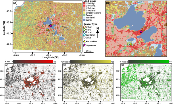
Figure 1. Map of the study area, Dane County WI. (a) NLCD land cover classification (Fry et al 2011), including sensor locations. (b) Close-up of Downtown Madison. (c)–(e) results of spectral unmixing analysis for % impervious, grass, and trees, respectively, calculated using the hybrid technique. Agricultural land use (cropland and grass/pasture), water and 2001–2011 land cover change are masked from (c) to (e).
Download figure:
Standard image High-resolution image2.2. Sensor data
Beginning in March 2012, 151 HOBO U23 Pro v2 temperature/RH sensors (Onset Computer Corporation, Bourne MA) were installed on utility and streetlight poles in and around Madison. 135 sensors were installed in March 2012, with an additional six sensors installed in October 2012 and ten more in August 2013. All sensors were equipped with radiation shields, installed at a height of 3.5 m, and logged instantaneous temperature every 15 min. Sensors were classified as Urban, Rural, Park, Lake, or Wetland at the time of installation. Specifically, urban sensors were defined as within the municipal limits of one of the cities or towns within the Madison metropolitan area (including Madison, Monona, Middleton, Sun Prairie, Fitchburg, Verona, Waunakee, and Stoughton), while rural sensors were outside of these boundaries. Park sensors were within municipal boundaries of a city or town, and inside an officially designated park; parks range in size from 1.7 to 520 ha, with a mean (median) size of 101 ha (39.2 ha). A full description of the sensor network, which is one of the most spatially dense and extensive in existence, can be found in Schatz and Kucharik (2014).
A detailed description of our approach for estimating SOS/EOS based on temperature data is described in appendix S1. In short, we used a heating and cooling degree day (HDD and CDD) approach developed by Richardson et al (2006) for sugar maple, which is the Wisconsin state tree and an important component of Madison's urban canopy. The HDD/CDD approach is based on the concept of thermal time and estimates the start and end of growing seasons based on cumulative temperature above/below a physiologically meaningful threshold (Cannell and Smith 1983, Fu et al 2014a).
As this approach represents only a single species and was developed in New Hampshire, we also used a permutation-based approach to quantify uncertainty associated with our estimate, in which temperature thresholds and other necessary parameters are randomly selected from a distribution in order to provide a range of values, from which both a mean and uncertainty can be estimated (Serbin et al 2014, Zipper and Loheide 2014). We selected a uniform distribution from −0.6 °C to 4 °C as our temperature threshold range for SOS thresholds for HDD accumulation, as this interval encompasses a range of vegetation, from cold-tolerant to warm-season, and these temperatures have been demonstrated as effective phenological predictors previously (Schwartz and Marotz 1986, Richardson et al 2006). As less data exists for the autumn phenological triggers, we varied our EOS threshold for CDD accumulation over the same 4.4 °C range centered on the 20 °C value reported by Richardson et al (2006) as most effective for sugar maple.
For each sensor and each growing season, cumulative HDDs beginning January 1 and CDDs beginning August 15 were used to identify the temperature-based SOS/EOS (SOST and EOST, respectively), and GSLT was calculated as EOST − SOST. The 2012 SOST is an exception to this, as the sensors were installed in late March and therefore temperature from a meteorological station at the University of Wisconsin-Madison Arboretum were adjusted for the UHI effect unique to each sensor and used prior to March 27. Differences between urban, park, and rural sensor classes were tested for statistical significance using a pairwise t-test with significance defined as p < 0.05.
2.3. Satellite data
A detailed description of the methodology for calculating phenology from remotely sensed data is presented in appendix S2. We collected all Landsat images of Madison WI (path 24, row 30) over the period 2003–2013 with < 40% cloud cover, for a total of 110 images (figure S1). Each image was atmospherically corrected using the LEDAPS toolchain (Masek et al 2006), cloud-masked using the FMASK utility (Zhu and Woodcock 2012), and clipped to the boundaries of Dane County. We used a double-logistic model (Zhang et al 2003, Fisher et al 2006) to calculate a composite remotely sensed SOS/EOS (SOSR/EOSR) based on five different vegetation indices and calculated GSLR as EOSR − SOSR.
It is important to note that this timestacking method produces a representative or average SOSR/EOSR/GSLR for the period 2003–2013 at each pixel, rather than SOSR/EOSR/GSLR for each individual growing season (Fisher et al 2006, Elmore et al 2012, Melaas et al 2013). Due to infrequent Landsat overpasses (figure S1) and common summer cloud cover in the area, using Landsat imagery over a smaller time period such as 2012–2014 for direct comparison with temperature-based method is not possible. However, satellites with more frequent overpasses (e.g. MODIS, AVHRR) have spatial resolutions an order of magnitude coarser, which would make studying the fine-scale impacts of the UHI on phenology impossible. While data fusion from multiple sensors shows promise at obtaining phenological estimates at high spatial and temporal resolution (e.g. Liang et al 2014), fusion approaches currently struggle when pixels have a mix of land cover types, and therefore are not well-suited to urban analysis (Walker et al 2012, Zhang et al 2013, Klosterman et al 2014).
To address potential problems associated with comparing 2003–2013 remotely sensed imagery with 2012–2014 temperature data, all pixels containing land use change between 2001 and 2011 (Jin et al 2013) were masked from analysis. Furthermore, we separately fit and estimated phenology using data from the complete Landsat period of record (1982–2013) and carried out all subsequent analysis to determine whether choice of the Landsat period has an impact on results. Only results using the 2003–2013 Landsat imagery are presented here, as using 1982–2013 data did not substantially impact either results or interpretation (data not shown).
2.4. Comparison between temperature-based and remotely sensed approaches
To compare remotely sensed and temperature-based phenology, we averaged SOSR, EOSR, and GSLR within a 500 m buffer surrounding each sensor, as this distance has been recommended as a zone of influence for sensor-based studies (Oke 2006) and previous work found that 500 m best describes local climate variability in our study area (Schatz and Kucharik 2014). Due to the different time periods of remotely sensed (2003–2013) and temperature-based (2012–2014) methods, it is important to note that a 1:1 relationship of phenological indicators between the methods is not expected, as the temperature regime controlling the timing of SOS/EOS varies interannually. However, temperature-based results show a consistent year-to-year relationship between SOST/EOST and impervious cover (discussed in section 3.1), indicating that the spatial patterns of UHI impact on meteorological conditions conducive to plant growth are consistent from year-to-year. Therefore, we hypothesize that a positive correlation reflecting these patterns exists between SOST/EOST from individual growing seasons and long-term average SOSR/EOSR. Our analysis focuses on the correlation and slope of the relationship between remotely sensed and temperature-based methods rather than bias between the two methods, as bias likely reflects the unique characteristics of the 2012–2014 growing seasons compared to the 2003–2013 average (see Ault et al 2013).
As a first-order attempt to quantify the impact of land cover on differences between remotely sensed and temperature-based growing season, we define three difference metrics. For each difference metric, a positive value indicates that remotely sensed estimates correspond to a longer growing season than would be predicted from meteorological data (e.g. SOSR < SOST, EOSR > EOST, and GSLR > GSLT):
- (1)SOSDiff = SOST_Norm − SOSR_Norm
- (2)EOSDiff = EOSR_Norm − EOST_Norm
- (3)GSLDiff = GSLR_Norm − GSLT_Norm
To account for the different temperature-based growing seasons (2012–2014) within a single model, we calculated normalized values of SOST, EOST, and GSLT (denoted SOST_Norm, EOST_Norm, and GSLT_Norm) by subtracting the yearly mean value across all sensors from each individual sensor's value, thus centering our data at 0 for all years. Similarly, we subtracted the overall mean value from each sensor's value for the remotely sensed metrics SOSR, EOSR, and GSLR to estimate SOSR_Norm, EOSR_Norm, and GSLR_Norm. Using this technique, there are three difference metrics for each sensor (once for each growing season).
To account for potential impacts of land use change across the interval over which Landsat results were averaged, we eliminated from analysis all pixels classified as changing land cover between 2001 and 2011 in the National Land Cover Dataset (NLCD) (Jin et al 2013). Furthermore, we repeated our analysis using SOSR and EOSR derived from a different Landsat time window (1982–2013) to check for the impacts of time domain selection on mean phenology, which had no substantial difference in results or interpretation (only 2003–2013 results shown below).
2.5. Land cover composition
We used two approaches to characterize the relative composition of impervious, tree, and grass cover at 30 m resolution (figures 1(b)–(d), both relying on spectral mixture analysis. Spectral mixture analysis is a widely used technique for estimating relative composition of different land cover classes by comparing the spectral signature of each pixel to spectra from user-defined reference endmembers (Small 2001, Wu and Murray 2003, Wu 2004, Buyantuyev et al 2007, Weng 2012). Inputs to both approaches were 30 cloud-free Landsat images collected between 2003 and 2013 with cropland and water masked (Gan et al 2014), and spectral mixture analysis was conducted in ENVI 5.0 (Exelis Visual Information Solutions, Boulder, Colorado) and constrained to a unit sum.
In the first approach (referred to as the SMA method), we performed a linear spectral mixture analysis, trained with areas of homogeneous cover manually selected in each of the three classes. In the second approach (referred to as the hybrid method), we use percent impervious cover from the NLCD (Xian et al 2011), a national-level impervious cover estimate widely used in the UHI literature (e.g. Georgescu et al 2012, 2013, Zhang et al 2014, Walker et al 2015, Schatz and Kucharik 2015, 2016). We then used spectral mixture analysis to differentiate between tree and grass cover for the remaining percent land cover in each pixel not accounted for by NLCD impervious estimates.
We assessed the accuracy of each method by comparing results to manually digitized 2013 Dane County imagery from the US Department of Agriculture's National Agricultural Imaging Program (NAIP). NAIP imagery was manually classified into 'birds-eye view' percent impervious, tree, and grass cover at 50 randomly selected 90 m × 90 m blocks, which were compared to 3 pixel-square blocks of Landsat-derived land cover (Wu and Murray 2003, Wu 2004, Gan et al 2014). Comparison between the two methods revealed only minor differences in results which did not alter overall interpretation, but a slightly better performance of the hybrid method; thus, results and analysis based on the hybrid method are reported in the main body text. Accuracy assessment results and a comparison of the two methods is presented in appendix S3.
3. Results and discussion
3.1. Temperature-based growing season
The temperature-based growing season shows a strong influence of the UHI (figures 2 and 3). Median urban sensor SOST is advanced by 0.8, 0.9, and 2.0 d relative to the rural sensors in 2012, 2013, and 2014, respectively, and urban EOST delayed by 4.2, 3.2, and 3.3 d. These changes in SOST and EOST lead to a statistically significant median increase in GSLT by 4.9–5.3 d in urban areas (figure 2).
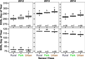
Figure 2. SOST and EOST based on degree-day technique aggregated by sensor class. Hinges are at the class median, boxes span the interquartile range (IQR), and whiskers span 1.5*IQR with outliers plotted as circles. Letters above boxes indicate statistically significant differences (p < 0.05) tested using pairwise t-test.
Download figure:
Standard image High-resolution image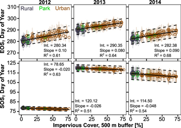
Figure 3. SOST and EOST based on degree-day technique, plotted as a function of impervious cover in the 500 m surrounding the sensor calculated using the hybrid method. Colors correspond to sensor type categories as shown in upper left panel. Points represent mean of 100 permutations and vertical lines one standard deviation around each point. Solid black line is a linear fit to means and dashed lines to ±1 standard deviation. All slopes and intercepts are significantly different from 0 (p < 0.05) using two-tailed t-test.
Download figure:
Standard image High-resolution imageThe changes in SOST and EOST are related most strongly to the percent impervious land surface cover (%I), a proxy for the density of the built environment, in the area surrounding the sensor (figure 3). We averaged %I within 500 m of each sensor, as local climate variability in our study area is best described at this distance (Schatz and Kucharik 2014), but changes in buffer radius (100–1000 m) do not substantially alter results (data not shown). Across all years, R2 for the %I–SOST/EOST relationships range from 0.51 to 0.68, indicating that physical urban density consistently explains over half of GSLT variability. Uncertainty estimates generated using our permutation-based approach show similar trends as a function of impervious cover, indicating that variability in temperature thresholds or degree day accumulation intended to represent a range of potential urban species does not alter the relationship between the UHI and phenology.
Phenological shifts when considering rural and urban endmembers, which we define as the minimum (0.7%) and maximum (76.1%) observed impervious cover within a 500 m buffer of all sensors, were even more extreme than shifts in median SOST/EOST. The urban endmember SOST was advanced by 1.5–3.7 d and EOST delayed by 6.0–7.9 d relative to the rural endmember. This represents a potential UHI-driven extension of the growing season by 8.0–10.5 d, or 4.7%–6.2% across our three study years.
The magnitude of UHI-driven changes in phenology are strongly determined by the prevailing weather conditions during seasonal transitions. The 2012 and 2014 SOST provide a useful contrast to explore this dynamic. In 2012, much of the US including Madison WI experienced anomalously high late winter temperatures leading to a record-setting 'false spring' (Ault et al 2013). This was driven by a regional, synoptic-scale warm front which elevated temperatures above physiologically important thresholds more or less simultaneously across urban and rural parts of our study area, and therefore the small temperature differences caused by the UHI had relatively little effect. In contrast, 2014 experienced a relatively cool spring, which meant that small (1 °C to 2 °C) increases in temperature due to the UHI were able to contribute a larger proportion of the degree day requirements to trigger the onset of spring. Therefore, the magnitude of urban impacts on SOST were ∼2.4 times as strong in 2014 compared to 2012, as measured by the difference in slopes between the two growing seasons (− 0.020 d/% in 2012 and − 0.048 d/% in 2014). This indicates that studies reporting UHI-driven increases in GSL on the basis of a single growing season (e.g. Schmidlin 1989, Zhang et al 2004) may not be generalizable across time without considering prevailing weather conditions during spring and fall transition periods.
Park sensors tended to have intermediate values of SOST and EOST between the urban and rural sensors, indicating that they likely experience both a UHI effect elevating temperatures above the rural surroundings and a park cool island (PCI) effect reducing temperature relative to their urban surroundings (Taha et al 1991, Spronken-Smith and Oke 1999, Upmanis and Chen 1999, Spronken-Smith et al 2000, Yu and Hien 2006, Feyisa et al 2014). The PCI leads to a subdued expression of the UHI and median park GSLT 1.7–3.2 d longer than rural sensors (p < 0.05 in 2013 and 2014) and 1.5–3.3 d shorter than urban GSLT (p < 0.01 all years). This subdued phenological response to the UHI in parks may be particularly beneficial for native and migratory species which rely on vegetation phenological events for survival (e.g. budburst), as urban parks are often viewed as refugia for species threatened by the urbanization process (Dobrowski 2011, Stagoll et al 2012).
3.2. Remotely sensed growing season
SOSR, EOSR, and GSLR are shown in figures 4(a), (c), (e). Patterns of urban and peri-urban land surface phenology are consistent with those observed in other studies, with earlier SOSR and later EOSR observed close to the center of the city (Fisher et al 2006). Due to the elimination of agricultural lands surrounding Madison from analysis, phenological estimates are much less dense outside the urban margin. However, it is evident that GSLR is shorter in rural landscape surrounding Madison, with several patches of longer GSLR corresponding to small outlying cities and towns. Areas that are predominantly wetland (e.g. northeast and south of Madison) have the shortest observed GSLR within our study domain, indicating that the growing season of naturally cool areas is well captured.
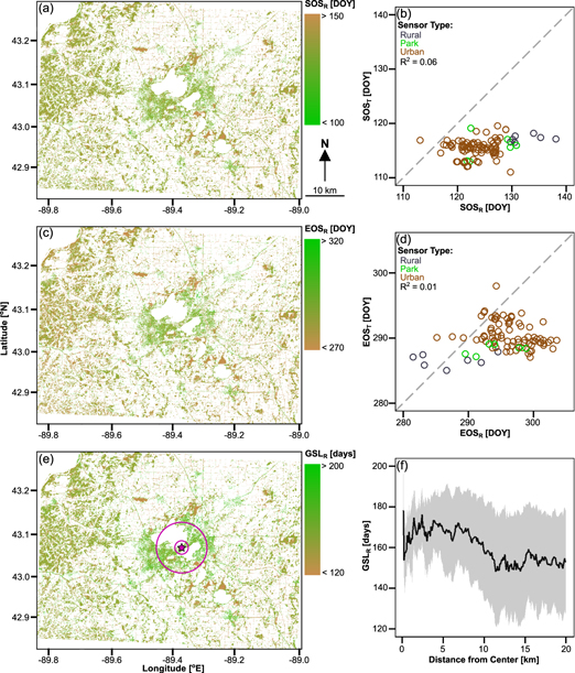
Figure 4. Remotely sensed estimates of (a) SOSR, (c) EOSR, and (e) GSLR with all agriculture, water, and failed fits masked (white areas). (b) and (d) compare SOSR to SOST and EOSR to EOST, respectively. In (b) and (d), SOSR and EOSR points represent the average SOS/EOS in a 500 m buffer surrounding the sensor as described in appendix S2; SOST and EOST represent the mean of the SOS/EOS from the 2013 and 2014 growing seasons at each sensor (2012 excluded due to false spring). (f) shows GSLR as a function of distance from the city center, which is noted as a purple star in (e). Purple circles in (e) represent 2 km (inner) and 7 km (outer) from city center. Black line in (f) represents the mean and gray shading one standard deviation of all pixels a given distance from center.
Download figure:
Standard image High-resolution imageAt the county scale, GSLR increases of ∼10–25 d are observed within ∼10 km from the city center (defined as the Wisconsin state capitol building; purple star in figure 4(e)) and maximum increases occur ∼2–7 km from the city center (figure 4(f); purple circles in figure 4(e)). These patterns exist due to the combined effects of the Madison lakes (suppressing GSLR within 2 km of the city center) and the urban–rural transition (occurring ∼6.5–11 km from the city center).
We believe that GSLR is suppressed within the 2 km closest to the city center due to a unique characteristic of Madison, which is that the densest parts of the city are on an isthmus between two lakes (figure 1). While these lakes visually dominate the landscape, previous work by Schatz and Kucharik (2014) has found that the lake's zone of influence on temperature is relatively small (100s of meters), and impacts of lakes on temperature decay exponentially with distance from the lakeshore. Therefore, the 2 km closest to the city center (equal to the half-length of the isthmus and shown as the inner purple circle in figure 4(e)) represents the area over which lakes contribute a larger proportional influence on temperature and phenology; however, previous work has shown the influence of the lakes on temperature is minor outside of this narrow zone on the isthmus (Schatz and Kucharik 2014).
Instead, the urban–rural transition represents the primary control over observed patterns in GSLR, a pattern similar that shown by Fisher et al (2007) in Providence RI and supporting recent work indicating that urban form determines the spatial extext of urban impacts on the thermal environment (Yang et al 2016). The city of Madison extends ∼6.5 km south from the city center, and ∼8–11 km on the east and west sides of town; therefore, the radial interval from ∼6.5 to 11 km distance represents the urban–rural transition zone. This transition is evident in figure 4(f), where we can see a decrease in GSLR over this approximate interval, and relatively static baseline rural GSLR at distances greater than 11 km. The decrease in GSLR over this urban–rural transition zone can be explained by two mechanisms. First, this transition is characterized by a decrease in impervious cover with increasing distance from the city center (figure 1). Based on the observed relationship between GSLT and impervious cover (section 3.1), the meteorological period suitable for vegetation growth is longer in urban areas with denser impervious cover and a warmer temperature regime, leading to a lower GSLR in the surrounding rural areas. Second, urban areas are often characterized by exotic, ornamental, or invasive vegetation (McKinney 2002, Niinemets and Peñuelas 2008), including non-native evergreen plants, which may be characterized by a longer growing season (Shustack et al 2009, Nemec et al 2011). Thus, we suggest that decreases in non-native vegetation moving outward from the city center contributes to the observed decrease in GSLR over the urban–rural transition zone and reinforces previously described temperature effects.
3.3. Comparison between remotely sensed and temperature-based metrics
While temperature-based and remotely sensed metrics show comparable patterns of longer growing seasons in urban Madison compared to the rural surroundings, when SOS/EOS are compared directly there is no statistically significant relationship between temperature-based and remotely sensed phenology at the individual sensor level (figures 4(b) and (d); R2 < 0.06). As noted in section 2.4, we did not expect there to be a 1:1 relationship between SOST/EOST (which represents the individual 2012–2014 growing seasons) and SOSR/EOSR (which represents the mean of the 2003–2013 growing seasons); rather, we hypothesized that there would be a significant positive correlation between the two methods due to persistent interannual temperature effects on phenology described in section 3.1, with a bias between methods due to the different sampling intervals. To study the drivers of differences between temperature-based and remotely sensed metrics, we introduced three difference metrics (SOSDiff, EOSDiff, GSLDiff) in section 2.4. For each difference metric, a positive value indicates that remotely sensed estimates correspond to a longer growing season than would be predicted from meteorological data (e.g. SOSR < SOST, EOSR > EOST, and GSLR > GSLT).
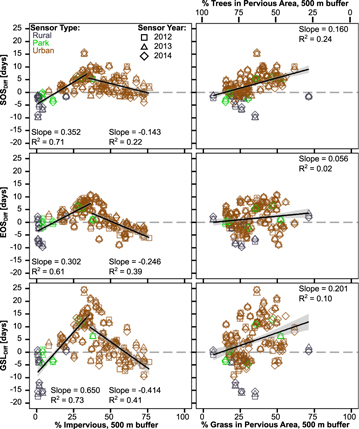
We find significant relationships between our different metrics and the land cover in the area surrounding each sensor (figure 5). Relationships between impervious cover (%I) and our difference metrics are best explained by a piecewise linear function, with a breakpoint determined as the %I which minimizes the sum of squared errors between model fit and difference metrics. Breakpoints are consistent across difference metrics at %I of 35% (SOSDiff), 37% (EOSDiff), and 36% (GSLDiff) (figure 5). Beneath this breakpoint, increasing %I is associated with a longer realized growing season relative to meteorological potential at a rate of 6.5 d/10%, with approximately even contributions from changes to SOSDiff and EOSDiff. Above this breakpoint, increasing %I is associated with a shorter growing season at a rate of 4.1 d/10%, with ∼2 times stronger effects on EOSDiff than SOSDiff.
Figure 5. Comparison of the difference metrics with land cover within a 500 m buffer of each sensor estimated using the hybrid method. Positive values on y axis indicate that the remotely sensed predictions of GSL are longer than the temperature threshold estimates. In right set of plots, % Grass and % Trees in Pervious Area must add up to 100 and reported slopes are based on % Grass. Plots exclude sensors with >75% masked pixels within a 500 m buffer. All relationships are statistically significant at p < 0.05.
Download figure:
Standard image High-resolution image
We attribute this piecewise pattern to two drivers: vegetation composition and urban stress regimes. First, moving outward from the city center, land cover transitions between the following classes: (Zone 1) high-density urban areas dominated by impervious cover, to (Zone 2) old neighborhoods with a thick urban canopy dominated by tree cover, to (Zone 3) recently developed areas with sparse urban canopies and a stronger grass signal, to (Zone 4) rural areas predominantly characterized by agriculture and trees (figures 1(c)–(e)). Sensors with peak difference metrics (30% < %I < 40%) are primarily in low-density urban areas (Zone 3) surrounding Madison, as well as outlying towns and villages, where grass cover is highest, and the other sensors making up the increasing limb (%I < 36%) are in rural areas or the urban outskirts (Zone 4), where most remaining natural vegetation is trees. Therefore, the increasing limb of the %I relationships represents an increase in the relative proportion of cold-tolerant urban turfgrass within vegetated areas (%G), which is typically green from shortly after snowmelt in the spring until the first winter snowfall, moving from Zone 4 into Zone 3. This is supported by a significant positive correlation between %G and SOSDiff (R2 = 0.24, p < 0.001), as well as a weakly positive correlation with EOSDiff (R2 = 0.02, p < 0.05) (figure 5). Overall, GSLDiff increases (i.e. the observable period of greenness grows longer relative to our temperature-based estimates) by 2 d for every 10% increase in %G, with ∼75% of that change occurring at the beginning of the growing season. The decreasing limb of the %I relationships, then, may also be partially explained by the decrease in grass cover associated with the transition from low-density urban areas surrounding Madison (Zone 3) to the higher-density areas closer to the city center (Zones 1 and 2) in which %G decreases.
Second, we suggest that the decreasing limb observed in %I relationships is may be due to increased water or pollutant stress in denser urban areas (Zones 1 and 2), which can lead to early onset of senescence and effectively decouples EOSR from meteorological conditions (Gratani et al 2000, Honour et al 2009, Sjoman and Nielsen 2010). This is supported by the observation that the slope of the decreasing relationship between %I and EOSDiff is approximately double the slope of the decreasing relationship between %I and SOSDiff. While our analysis does not consider irrigation, variability in water available to plants as a result of urban irrigation (e.g. Pataki et al 2011, Bijoor et al 2012, Vico et al 2014) may further decouple EOSR from EOST, e.g. by allowing irrigated vegetation to remain green during drought while non-irrigated vegetation may senesce.
While our analysis is conducted at a plant functional type level (e.g. grass versus trees), previous field- and plot-based studies have shown that phenological response to temperature varies at the species level (Bradley et al 1999, Chuine 2000, Primack et al 2004, Morin et al 2009, Vitasse et al 2009, Jochner et al 2013). A further complication is that non-native vegetation is common to urban areas and may be associated with earlier greening in the spring and a concomitantly longer GSLR, as discussed in section 3.2 (McKinney 2002, Niinemets and Peñuelas 2008, Shustack et al 2009, Nemec et al 2011). If we assume that non-native vegetation common to urban areas has a longer growing season than native vegetation, this would cause an earlier SOST (downward shift of urban sensors in figure 4(b)) and a later EOST (upward shift of urban sensors in figure 4(d)), both of which would improve the correlation between temperature-based and remotely sensed phenological metrics.
While our temperature-based method accounts for potential variability in species-specific biological responses to thermal conditions by varying input parameters to our HDD/CDD equations (see appendix S1), this technique implicitly assumes a random and homogeneous distribution of all species by equally weighting all parameter combinations when calculating the mean SOST/EOST for each sensor. To account for spatial variability in species composition, the fitting parameters in table S1 could be 'tuned' to maximize agreement between SOST/SOSR and EOST/EOSR at each sensor (e.g. Fisher et al 2007); however, this approach would assume that temperature is the only factor contributing to spatial variability in phenology, whereas factors such as intra-species variability in response to photoperiod or environmental stressors may contribute to spatial variability in phenology (Gratani et al 2000, Saxe et al 2001, Schaber and Badeck 2003, Honour et al 2009, Caffarra et al 2011). Urban pixels are typically mixes of the built environment and vegetation (Gao et al 2006, Klosterman et al 2014, Lazzarini et al 2015, Walker et al 2015), leading to greater variability in both land cover and phenology than natural areas (Buyantuyev and Wu 2012).
These results provide the first synthesis of remotely sensed phenology with a dense ground-based urban temperature sensor network, and highlight a disagreement between the two methods which is associated with fine-scale variability in land cover. As previous work has reported substantial bias between remotely sensed and observed phenology, SOSR/EOSR are typically used to compare the relative timing of phenological events, rather than the exact dates (White et al 2009, Cong et al 2012, Xu et al 2014). However, here we show that remotely sensed observations of variability in land surface phenology cannot be used as a proxy for UHI intensity, as the vegetative response to meteorological conditions is dependent on the highly variable land cover at and surrounding a point. Even when focusing on the response of a single plant functional type to the UHI, such as forests in Fisher et al (2006) and Elmore et al (2012), we find that land cover (particularly %I) surrounding a pixel alters realized GSL and needs to be considered before conclusions can be drawn about the strength of the UHI. These results extend previous work done at larger spatial scales showing a disconnect between meteorological conditions and phenological response (Fisher et al 2007) and indicates that local processes, particularly land cover composition, must be considered as an important control over the vegetative response to changes in land cover in addition to changes in climate.
4. Conclusions
Overall, we find that the UHI has a significant impact on urban phenology with intra-urban variability over fine spatial scales in response to local land cover composition. Across all growing seasons, we find that the UHI leads to statistically significant increases GSLT in urban areas, with a PCI effect partially counteracting the UHI impacts on GSLT and a small and relatively localized lake effect near the lakeshore (figure 2). Impervious cover in the area surrounding temperature sensors explains ∼50%–70% of observed variability in both SOST and EOST (figure 3). However, the magnitude of the UHI impact on phenology varies interannually, and is driven by the prevailing regional weather conditions during the spring/fall transitional seasons. As such, we conclude that studies based on a single year of data are likely not generalizable to other growing seasons, though spatial patterns are likely to be consistent across years.
Comparison between remotely sensed and temperature-based phenology reveals that there is no relationship between remotely sensed and temperature-based SOS, EOS, or GSL at the individual sensor level (figures 4(b) and (d); R2 < 0.06). We attribute this to the impacts of impervious cover and vegetation type within the zone of influence surrounding each sensor on the realized phenological response to meteorological conditions. Furthermore, our results demonstrate that remotely sensed phenology cannot be used as a simple proxy for UHI intensity due to potential confounding effects of local land cover composition. These results represent a first step towards better understanding local drivers of phenological variability including environmental stressors, photoperiod, and plant species and functional type variability, which has been suggested by previous studies (Cleland et al 2007).
As impervious surfaces are the defining characteristic of cities worldwide and our results show that local-scale impervious cover represents the dominant control over observed intra-urban variability in phenology, we expect these process-based conclusions to be broadly applicable to other cities, particularly in temperate climates. This study represents the first comparison between temperature-based phenological estimates from an urban sensor network and remotely sensed estimates; as urban meteorological networks become more common (e.g. Smoliak et al 2015), future work should focus on understanding the mechanisms by which land cover influences the vegetative response to urban warming and implications of UHI-induced variability in phenology for water, energy, and nutrient cycling.
Acknowledgments
SCZ, JS, CJK, and SPL are funded by the National Science Foundation Water Sustainability & Climate Program (DEB-1038759) and the North Temperate Lakes Long-Term Ecological Research Program (DEB-0822700). PT and AS acknowledge support from the NASA Applied Science program (NNX14AC36G). Tedward Erker provided helpful discussion regarding urban vegetation. The University of Wisconsin-Madison Center for High Throughput Computing (CHTC) provided computational resources for satellite image processing. We thank our community partners for use of their streetlight and utility poles: Madison Gas & Electric (RJ Hess), Alliant Energy (Jeff Nelson), the City of Madison (Dan Dettmann), Madison City Parks (Kay Rutledge), Sun Prairie Utilities (Rick Wicklund; Karl Dahl), Waunakee Utilities (Dave Dresen), the UW-Madison Arboretum (Brad Herrick), the City of Fitchburg (Holly Powell), UW-Madison (Kurtis Johnson), and Dane County (Darren Marsh). Temperature data are available by contacting JS or CJK. We appreciate the comments of two anonymous reviewers, which significantly improved the quality of the manuscript.