

Abstract
We project that within the next two decades, half of the world's population will regularly (every second summer on average) experience regional summer mean temperatures that exceed those of the historically hottest summer, even under the moderate RCP4.5 emissions pathway. This frequency threshold for hot temperatures over land, which have adverse effects on human health, society and economy, might be broached in little more than a decade under the RCP8.5 emissions pathway. These hot summer frequency projections are based on adjusted RCP4.5 and 8.5 temperature projections, where the adjustments are performed with scaling factors determined by regularized optimal fingerprinting analyzes that compare historical model simulations with observations over the period 1950–2012. A temperature reconstruction technique is then used to simulate a multitude of possible past and future temperature evolutions, from which the probability of a hot summer is determined for each region, with a hot summer being defined as the historically warmest summer on record in that region. Probabilities with and without external forcing show that hot summers are now about ten times more likely (fraction of attributable risk 0.9) in many regions of the world than they would have been in the absence of past greenhouse gas increases. The adjusted future projections suggest that the Mediterranean, Sahara, large parts of Asia and the Western US and Canada will be among the first regions for which hot summers will become the norm (i.e. occur on average every other year), and that this will occur within the next 1–2 decades.
Export citation and abstract BibTeX RIS

Original content from this work may be used under the terms of the Creative Commons Attribution 3.0 licence. Any further distribution of this work must maintain attribution to the author(s) and the title of the work, journal citation and DOI.
1. Introduction
Global mean temperatures have increased since the late 19th century (Hartmann et al 2013). The warming has been accompanied by an increase in extreme warm temperatures (IPCC 2007) and an increase in the occurrences of hot days (Seneviratne et al 2014). Recent heat waves such as those in Western Europe (2003), Russia (2010) and the Southern Great Plains of the US (2011) have clearly demonstrated their large negative impacts on human health, ecosystems, agriculture and economy (see Coumou and Rahmstorf 2012, for an overview). For the purpose of climate change adaptation and disaster management, it is important to assess whether there have been changes in the frequencies of such events and how they might change in the future. It is also important to understand the causes of the changes.
The increase in the magnitude and likelihood of extremely hot temperatures has been attributed to the human influence on the climate system (e.g. Christidis et al 2011, Zwiers et al 2011, Bindoff et al 2013, Min et al 2013, Wen et al 2013, Christidis et al 2015b, Kim et al 2016). Human influence may have resulted in a four-fold increase in the probability of a year during 2000–2009 being warmer than the hottest year of the 20th century in almost all regions of the globe (Christidis et al 2012). The increase in hot temperatures is projected to continue in the future (Jones et al 2008, Morak et al 2013). Jones et al (2008) estimated that in the northern hemisphere, a hot summer that occurred once every 10 years in the past will occur in 1 out of 2 years before 2018. Mora et al (2013) projected that the annual temperature over half of the global area will become higher than the highest 1860–2005 temperatures starting between 2047 and 2069.
Projected future changes in the climate are typically based on climate model simulations (e.g. Mora et al 2013). However, a climate model that underestimates the past temperature increase may also underestimate the future increase. Conversely, a model that overestimates the past change could be expected to overestimate the future change. It is reasonable to assume that the fractional errors in projecting future temperature changes are linearly related to those in simulating past temperature changes, and therefore to use past observations to constrain future projections. Under a linear regression framework, the scaling factor that best matches historical observations with model simulations has been used to scale future projections (Allen et al 2000, Stott and Kettleborough 2002, Lee et al 2006, Stott and Forest 2007).
Limiting the average global surface temperature increase to 2 K over the pre-industrial average has been used as a mitigation target in international climate policy discussions 'to avoid dangerous anthropogenic interference in the climate' (Randalls 2010). However, such a target for a global mean temperature increase can be rather abstract for policy makers for two reasons: first, it is difficult to link a global warming target to local and regional impacts that many policy makers are more concerned about. Second, the Earth is expected to warm unevenly, e.g. land areas warm faster than oceans, and warming rates in different parts of the land surface differ (IPCC 2013).
Hot summers defined as summers with higher mean temperatures than during the historically hottest summer over a region can be an attractive reference for future climate change projection because their negative effects have been experienced. Changing probabilities of temperatures at historically high levels have been studied in earlier work; Christidis et al (2015b), for example, estimated the change in the likelihood of very warm years and seasons as simulated by climate models and constrained by global space–time patterns of observed temperature anomalies. Sun et al (2014) estimated that anthropogenic influence has caused temperatures as observed in the summer of 2013 in Eastern China to be 60 times more likely at present than under pre-industrial conditions. They projected that the region will experience similarly hot summers even more frequently in the future, with 50% of summers being hotter than the 2013 summer within two decades.
Here we provide projections of the likelihood of hot summers for different parts of the world. These projections are constrained by observations, using a method similar to Sun et al (2014) and based on regularized optimal fingerprinting (ROF, Ribes et al 2013). We further project the fraction of the world's population that would be exposed to these hot summer temperatures—a measure relevant for adaptation purposes.
2. Methods and data
2.1. Methods
We use detection and attribution analysis (e.g. Allen and Stott 2003, Ribes et al 2013) to assess whether climate model simulations of summer temperatures are consistent with observations. We first average land-surface temperatures over three summer months and over the regions outlined in figure 1(A). We then estimate the factors by which the model simulated response to anthropogenic and natural forcing (ALL) should be scaled to best match the observations. These scaling factors are obtained by regressing observations onto the expected climate responses to external forcings, i.e. the signals represented by the multi-model ensemble mean of climate simulations under the respective forcings. We use the standard total least square based optimal detection method (Allen and Stott 2003) for the detection and attribution analysis. This method takes noise in the model-simulated climate response that arises from internal climate variability into account. This requires estimates of the climates internal variability, which we obtain following the Ribes et al (2013) approach that uses a regularized estimates of the covariance matrix estimator in place of standard sample covariance matrices as regularization improves the covariance matrix estimates (see discussion in Ribes et al 2013) and obviates the need for adhoc regularization, such as through the EOF truncation approach that has often been used in the past.
The goodness of fit of the regression models is tested using a residual consistency check (Allen and Tett 1999, Ribes et al 2013). Figure 1(B) illustrates the best-estimate and the 5th and 95th percentile of the resulting ALL scaling factors for three selected regions. The signal is detected in the observations if the 90% confidence interval lies above zero. If the confidence intervals for the scaling factors include unity, the magnitudes of model-simulated and observed changes are comparable. If the scaling factors are larger than unity, the model simulated response is underestimated, and if they are smaller than unity, overestimated. We also perform a detection analysis using the climate response to natural (NAT) forcing alone, as well as to anthropogenic (ANT, obtained from ALL-NAT) and NAT forcing simultaneously (see figure D1 for all regions).
The best estimate of climate response to external (ALL) forcing in the observations is obtained by multiplying the model simulated response by the scaling factors. This is removed from the observations, and the residual is taken to represent natural variation of the climate without the influence of external forcings (see figure 1(C)).
We also use the ALL scaling factors to adjust the signals from historical ALL and future representative concentration pathway (RCP) simulations (figure 1(D)). The 380 samples of noise from pre-industrial simulations are added to these observational-constrained signals to produce multiple realizations of reconstructed and projected future temperature changes. Christidis et al (2012, 2015b) used a similar method, but with a single scaling factor obtained from a global space–time temperature pattern that was regionally resolved. By using scaling factors obtained for individual regions, we constrain signals only with information from the respective regions, which allows closer adjustment to regional differences between observed changes and signals, but also means that the uncertainty in the scaling factors is larger due to the averaging over smaller regions.
The proportion of reconstructed time series with temperature anomalies greater than the observed hottest temperature anomaly is referred to as the probability of exceedance (P1, see figure 1(D)), or as the probability of a hot summer. A similar probability (P0) is computed for the 380 pieces of control simulations. The fraction of attributable risk

is then computed for each region. The FAR lies between −Inf and 1. A negative value indicates that an event becomes rarer due to anthropogenic forcing, while a positive value indicates that the event becomes more frequent.
Lastly, we define the year after which the probabilities of a hot summer P1 are continuously larger than 50% and 90%. Each year, the population of the region for which this is the case is summed up to obtain time series of population exposure to hot summers.
2.2. Temperature data from models and observations
The observational data are the University of East Anglia Climatic Research Unit gridded global land-surface temperature anomalies (CRU version 3.21, Mitchell and Jones 2005). Climate model simulations were obtained from the Coupled Model Intercomparison Project phase 5 (CMIP5) multi model ensemble (Taylor et al 2012) and are listed in tables A.1 and A.2. We consider historic simulations under ALL and NAT forcings. For future projections, we include simulations from two emission scenarios—RCP4.5 and RCP8.5. The RCP8.5 assumes radiative forcing to be 8.5 W m−2 by 2100 (Riahi et al 2011, van Vuuren et al 2011). The reduction in emissions necessary to limit the forcing to this level is supposed to be reached with air quality legislation but without a strict climate policy. The RCP4.5 has a target radiative forcing of 4.5 W m−2 and requires, for example, a decline in overall energy and fossil fuel use and a substantial increase in renewable energy forms (Thomson et al 2011). The increase in the global mean temperature is estimated to be 4.9 and 2.4 K above pre-industrial levels by 2100 under the RCP8.5 and RCP4.5 scenarios, respectively (Rogelj et al 2012).
Our ensemble consists of 54 ALL simulations, 45 NAT simulations, and 15 RCP4.5 and RCP8.5 simulations. When constructing time series over the past and future, we selected only model members from ALL simulations that also produced RCP runs (indicated with ALLrec in table A.1). We conduct the detection and attribution analyzes based on the period 1950–2012 (63 years) and provide future projections for the period 2013–2069 (57 years). Fifty-one multi-year control simulations from various models are also used for the estimation of internal variability. Overall, these control simulations provide 380 chunks of data which are of the same length as the historical data (63 years).
We interpolate all data onto a 5 × 5° grid and mask the historical and control simulations to mimic availability of the CRU data. We then compute the summer mean temperatures by averaging monthly values of the three summer months (June–August for the northern hemisphere and December–February for the southern hemisphere). For the observations and ALL and NAT simulations, anomalies are calculated relative to the individual simulations' average over 1950–1984; anomalies are similarly calculated relative to the year 0–34 average in the case of the control simulations. The anomalies for each RCP simulation are calculated relative to the respective historical ALL simulation (1950–1984). Finally, we average the anomalies over large regions (see figure 1(A)) with the same region boundaries as used in the Special Report on Extremes (IPCC SREX report, Seneviratne et al 2012). The detection and attribution analysis is performed on 3 year mean series.
2.3. Population
Projections of gridded population data for the years 2000–2100 are obtained from the GGI Scenario Database developed at the International Institute for Applied System Analysis (IIASA, Riahi and Nakicenovic 2007, scenario A2, available at http://iiasa.ac.at/Research/GGI/DB/). The original data is available at a time-step of 10 years. We obtain annual values by linearly interpolating the decadal values.
3. Results and comparison to other studies
3.1. Contribution of external forcing to past temperature maxima
For time series of global-averaged summer temperatures, the responses to ALL and NAT forcing are detected in the observations. In all 26 regions except for North Australia, the responses to ALL forcing are detected, while the response to natural forcing alone is only detected in 11 out of 26 regions (figure D1).
Not detecting the responses to ALL forcing in observed changes—as is the case in North Australia—indicates that the ensemble mean of the simulations under ALL forcing does not match observations well. In North Australia, observed summer temperatures show only a very small increasing trend (figure D2). For the sub-period of 1979–2010, Li et al (2013) even report a cooling trend over the region and suggest that the cooling is due to the increase in North Australian summer rainfall and surface evaporation. The reason for the positive trend in precipitation is still unclear, although Li et al (2013) suggest that it is linked to an anomalous Gill-type cyclone response to increasing sea surface temperatures in the tropical Western Pacific. While such variability is present in observations and thus mask the response to ALL forcing, ensemble averaging would have largely removed the influence of internal variability in the ensemble mean of ALL simulations, leaving essentially only the forced response. Thus a discrepancy between observations and the ALL signal in a region strongly affected by low frequency variability is not implausible despite strong evidence of the ALL influence at the global scale and in most other regions.
The confidence intervals for the ALL scaling factors include unity in most cases, indicating a good match between models and observations in general. The residual consistency checks indicate no evidence of too little model variability. In 21 regions, the model-simulated variability is consistent with the regression residuals. In the remaining 5 regions, the simulated variability is too large. Larger variability in model simulations increases the width of the confidence interval for the scaling factor, making the detection results more conservative. We therefore include all regions in the subsequent analyzes.
Column 2 in table B.1 lists the historically hottest summers for each region. By multiplying these years' model simulated response under ALL forcing with the ALL scaling factor (see figure 1(C)) for each region, we obtain the temperature anomaly attributable to external forcing (figure 2). The attributable temperature anomalies have a mean of 0.59 K with an interquartile range of 0.33–0.73 K across the regions. The highest attributable temperature anomalies of 1.59, 1.29 and 1.43 K appear in the Mediterranean, North Africa and the Middle East, respectively (regions 13, 14, 19, figure 2 and table B.1). Their temperature anomalies relative to the 1950–1984 mean in the absence of external influences are estimated to be 0.47, 0.34 and 0.47 K, respectively. These three regions are also among the regions with the largest observed summer temperature increases over the past few decades (figure D2).
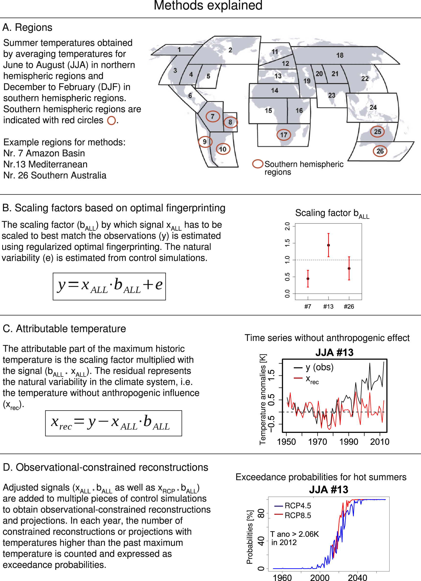
Figure 1. Method explained on the example of the Amazon Basin, the Mediterranean and Southern Australia.
Download figure:
Standard image High-resolution image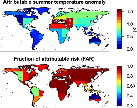
Figure 2. Summer temperature attributable to external forcing (top) and fraction of attributable risk (FAR, bottom) for summer temperature in the year with maximum historic summer temperature anomaly (see table B.1). The FAR is calculated from FAR = 1 –P0/P1 with P0 the probability of hot summers without any external forcing, and P1 the respective probability in simulations with external forcing.
Download figure:
Standard image High-resolution imageIn all regions except North Australia, the influence of external forcing on summer temperatures has become obvious over the last 30 years (figure D2). This has resulted in an increase in the occurrence probability of hot summers (supplementary figure S1), presented as the FAR in table B.1 and figure 2. Table B.1 also presents estimates of the uncertainty in the FAR (for explanations, see appendix
3.2. Timing of frequent hot summers
The year beyond which a region is projected to regularly experience hot summers is shown in figure 3. The timing represents the year after which the probability of a hot summer is higher than 50% (top) and 90% (bottom), respectively, in every subsequent year (for probability time series, see figure S1). This is synonymous with an occurrence frequency of 1 in 2 and 9 in 10 years, respectively, which we will also refer to as 'the norm' and 'most years', respectively (see table 1). As our analyzes extend only to the year 2069, 'every subsequent year' strictly means up to the end of our data record. The possibility that the probability for a hot summer after 2069 is below the thresholds cannot be ruled out completely, but is highly unlikely under the RCP4.5 and RCP8.5 pathways given that the projected warming is essentially irreversible on human time scales (Solomon et al 2009) . Note that we show results for both RCP4.5 and RCP8.5, but only discuss those for RCP4.5 in detail .

Figure 3. Year beyond which the probability of hot summers is larger than 50% (top) and 90% (bottom) estimated from observationally constrained reconstructions based on RCP4.5 (left) and RCP8.5 (right) simulations. Note that the years are determined from the reconstructions combining past and future simulations (see figure S1), and if a date before 2013 is shown, it has been determined from historical simulations.
Download figure:
Standard image High-resolution imageTable 1. Terms used for likelihood and recurrence rates.
| Occurrence probability | Years with | Alternative |
|---|---|---|
| per year | occurrence | terminology |
| >90% | > 9 out of 10 | Most summers |
| >50% | > 1 out of 2 | Being the norm |
Table A.1. List of model simulations used for ALL, ALL for reconstruction-based probabilities, NAT and RCPs experiments.
| Model | Run | ALL | ALL (rec) | NAT | RCPs | Model | Run | ALL | ALL (rec) | NAT | RCPs |
|---|---|---|---|---|---|---|---|---|---|---|---|
| CanESM2 | r1i1p1 | x | x | x | x | GISS-E2-H | r3i1p1 | x | x | ||
| CanESM2 | r2i1p1 | x | x | x | x | GISS-E2-H | r4i1p1 | x | x | ||
| CanESM2 | r3i1p1 | x | x | x | x | GISS-E2-H | r5i1p1 | x | x | ||
| CanESM2 | r4i1p1 | x | x | x | x | GISS-E2-H | r6i1p1 | x | |||
| CanESM2 | r5i1p1 | x | x | x | x | GISS-E2-H | r6i1p3 | x | |||
| CNRM-CM5 | r10i1p1 | x | GISS-E2-H | r2i1p3 | x | ||||||
| CNRM-CM5 | r1i1p1 | x | x | x | x | GISS-E2-H | r3i1p3 | x | |||
| CNRM-CM5 | r2i1p1 | x | x | GISS-E2-H | r4i1p3 | x | |||||
| CNRM-CM5 | r3i1p1 | x | x | GISS-E2-H | r5i1p3 | x | |||||
| CNRM-CM5 | r4i1p1 | x | x | GISS-E2-R | r1i1p1 | x | x | x | x | ||
| CNRM-CM5 | r5i1p1 | x | x | GISS-E2-R | r1i1p3 | x | x | x | x | ||
| CNRM-CM5 | r6i1p1 | x | GISS-E2-R | r2i1p1 | x | x | |||||
| CNRM-CM5 | r7i1p1 | x | GISS-E2-R | r2i1p3 | x | x | |||||
| CNRM-CM5 | r8i1p1 | x | x | GISS-E2-R | r3i1p1 | x | x | ||||
| CNRM-CM5 | r9i1p1 | x | GISS-E2-R | r3i1p3 | x | x | |||||
| CSIRO-Mk3-6-0 | r1i1p1 | x | GISS-E2-R | r4i1p1 | x | x | |||||
| CSIRO-Mk3-6-0 | r2i1p1 | x | GISS-E2-R | r4i1p3 | x | x | |||||
| CSIRO-Mk3-6-0 | r3i1p1 | x | GISS-E2-R | r5i1p1 | x | x | |||||
| CSIRO-Mk3-6-0 | r4i1p1 | x | GISS-E2-R | r5i1p3 | x | x | |||||
| CSIRO-Mk3-6-0 | r5i1p1 | x | GISS-E2-R | r6i1p3 | x | ||||||
| EC-EARTH | r12i1p1 | x | x | x | HadGEM2-ES | r1i1p1 | x | ||||
| EC-EARTH | r2i1p1 | x | x | x | HadGEM2-ES | r2i1p1 | x | ||||
| EC-EARTH | r7i1p1 | x | HadGEM2-ES | r3i1p1 | x | ||||||
| EC-EARTH | r8i1p1 | x | x | x | HadGEM2-ES | r4i1p1 | x | ||||
| EC-EARTH | r9i1p1 | x | x | x | IPSL-CM5A-LR | r1i1p1 | x | ||||
| GFDL-CM2p1 | r10i1p1 | x | IPSL-CM5A-LR | r2i1p1 | x | ||||||
| GFDL-CM2p1 | r1i1p1 | x | IPSL-CM5A-LR | r3i1p1 | x | ||||||
| GFDL-CM2p1 | r2i1p1 | x | IPSL-CM5A-MR | r1i1p1 | x | ||||||
| GFDL-CM2p1 | r3i1p1 | x | IPSL-CM5A-MR | r2i1p1 | x | ||||||
| GFDL-CM2p1 | r4i1p1 | x | IPSL-CM5A-MR | r3i1p1 | x | ||||||
| GFDL-CM2p1 | r5i1p1 | x | MRI-CGCM3 | r1i1p1 | x | x | x | ||||
| GFDL-CM2p1 | r6i1p1 | x | MRI-CGCM3 | r2i1p1 | x | ||||||
| GFDL-CM2p1 | r7i1p1 | x | MRI-CGCM3 | r3i1p1 | x | ||||||
| GFDL-CM2p1 | r8i1p1 | x | NorESM1-M | r1i1p1 | x | x | x | ||||
| GFDL-CM2p1 | r9i1p1 | x | NorESM1-M | r2i1p1 | x | ||||||
| GISS-E2-H | r1i1p1 | x | x | x | x | NorESM1-M | r3i1p1 | x | |||
| GISS-E2-H | r2i1p1 | x | x | Total | 54 | 15 | 45 | 15 | |||
Table A.2. Names of control runs used for internal variability estimates and temperature reconstructions.
| Number | Number | Number | Number | ||||
|---|---|---|---|---|---|---|---|
| Model | Run | of years | of chunks | Model | Run | of years | of chunks |
| ACCESS1-0 | r1i1p1 | 500 | 7 | GISS-E2-H | r1i1p3 | 530 | 8 |
| ACCESS1-3 | r1i1p1 | 500 | 7 | GISS-E2-H | r1i1p1 | 1770 | 12 |
| bcc-csm1-1 | r1i1p1 | 500 | 7 | GISS-E2-H-CC | r1i1p1 | 250 | 3 |
| bcc-csm1-1-m | r1i1p1 | 400 | 6 | GISS-E2-R | r1i1p141 | 1162 | 18 |
| BNU-ESM | r1i1p1 | 559 | 8 | GISS-E2-R | r1i1p142 | 100 | 1 |
| CanESM2 | r1i1p1 | 995 | 15 | GISS-E2-R | r1i1p1 | 1200 | 13 |
| CCSM4 | r1i1p1 | 500 | 7 | GISS-E2-R | r1i1p2 | 530 | 8 |
| CCSM4 | r2i1p1 | 155 | 2 | GISS-E2-R | r1i1p3 | 530 | 8 |
| CCSM4 | r3i1p1 | 120 | 1 | GISS-E2-R-CC | r1i1p1 | 250 | 3 |
| CESM1-BGC | r1i1p1 | 500 | 7 | HadGEM2-CC | r1i1p1 | 240 | 3 |
| CESM1-CAM5 | r1i1p1 | 320 | 5 | HadGEM2-ES | r1i1p1 | 240 | 9 |
| CESM1-FASTCHEM | r1i1p1 | 222 | 3 | inmcm4 | r1i1p1 | 590 | 7 |
| CESM1-WACCM | r1i1p1 | 200 | 3 | IPSL-CM5A-LR | r1i1p1 | 920 | 15 |
| CMCC-CESM | r1i1p1 | 277 | 4 | IPSL-CM5A-MR | r1i1p1 | 300 | 4 |
| CMCC-CM | r1i1p1 | 330 | 5 | IPSL-CM5B-LR | r1i1p1 | 300 | 4 |
| CMCC-CMS | r1i1p1 | 500 | 7 | MIROC-ESM | r1i1p1 | 630 | 10 |
| CNRM-CM5 | r1i1p1 | 850 | 13 | MIROC-ESM-CHEM | r1i1p1 | 255 | 4 |
| CSIRO-Mk3-6-0 | r1i1p1 | 500 | 7 | MIROC4h | r1i1p1 | 100 | 1 |
| EC-EARTH | r1i1p1 | 452 | 7 | MIROC5 | r1i1p1 | 670 | 10 |
| FGOALS-g2 | r1i1p1 | 900 | 14 | MPI-ESM-LR | r1i1p1 | 1000 | 15 |
| FGOALS-s2 | r1i1p1 | 500 | 7 | MPI-ESM-MR | r1i1p1 | 1000 | 15 |
| FIO-ESM | r1i1p1 | 800 | 12 | MPI-ESM-P | r1i1p1 | 1155 | 18 |
| GFDL-CM3 | r1i1p1 | 500 | 7 | MRI-CGCM3 | r1i1p1 | 500 | 7 |
| GFDL-ESM2G | r1i1p1 | 500 | 7 | NorESM1-M | r1i1p1 | 500 | 7 |
| GFDL-ESM2M | r1i1p1 | 500 | 7 | NorESM1-ME | r1i1p1 | 252 | 4 |
| GISS-E2-H | r1i1p2 | 530 | 8 | TOTAL | 390 |
Many northern hemispheric regions are projected to experience hot summers in 1 out of 2 years within a decade, and 9 out of 10 summers by 2040 (figure 3). Climate change has already impacted these regions in the past (Jones et al 2008, Christidis et al 2015b). Our analysis suggests that the Sahara region is the first to experience higher than historic summer temperature maxima—in 9 out of 10 summers within 15 years. The region exhibits a very strong warming trend and relatively small natural variability (figure D2). In Eastern Asia (region 22), we find that 1 out of 2 summers is projected to be hot by around 2020, comparable to the results from Sun et al (2014) for Eastern China (2025). Other areas for which hot summers are projected to soon become the norm are the Mediterranean region (around 2025), large parts of Asia (before 2025) and the Western US/Canada (2030, figure 3). These early dates are consistent with the strong summer temperature responses to climate change in these regions as documented in the IPCC 4th assessment report (AR4). The report shows that the median temperature response in the Sahara and the 'Southern Europe and Mediterranean' region are among the largest for the summer months (IPCC 2007 and table D.1). Jones et al (2008) also find a large increase in the occurrence probabilities in the Sahara and the Mediterranean regions in response to anthropogenic forcing, with a 1 in 10 year-event to become a 6 in 10 year and 7 in 10 year- event (or a FAR value of 0.83 and 0.86), respectively.
Our temperature threshold for hot summers in the Mediterranean is higher than the June–August average of the heat-wave summer of 2003. Such temperature extremes are projected to become the norm by 2025, and very few summers will be colder than that after 2035. The likelihood of hot summers in Europe has been studied extensively. Schar et al (2004) for example analyzed the temperature at the end of the twenty-first century simulated by a regional climate model and found that 1 in 2 summers would be as warm or warmer than the 2003 summer. Stott et al (2004) report a hundredfold increase in the expected frequency of 2003-type summers by the mid-twenty-first century, and Christidis et al (2015a) suggest that the human influence on this frequency has been underestimated.
3.3. Population exposure to hot future summers
The percentage of regions and population living in regions where summers are projected to be hot in 1 out of 2 (full lines) and 9 out of 10 years (dashed lines) are illustrated in figure 4. The timeseries are based on probabilities calculated from the observationally constrained projections. We ask the question: When are hot summers projected to be so widespread that half of the population regularly experiences summers (i.e. 1 in 2) that are hotter than any summer of the past? Under the moderate emission scenario RCP4.5, more than half of the world's population is projected to experience a hot summer in 1 out of 2 years within 20 years. If greenhouse gas emissions continue to rise throughout the 21st century (RCP8.5), this is projected to occur in just over a decade. The time at which half the world's regions are projected to be affected occurs only slightly later, which indicates that regions affected first have a somewhat smaller proportion of the global population. Just after 2050, nearly the entire population and over 70% of all regions are projected to be exposed to hot summers in 1 out of 2 years under RCP4.5.

Figure 4. Percentage of world regions (left) and population (right) that experience hot summers with a probability of over 50% (full lines) and 90% (dashed lines) in all subsequent years. Results are shown for reconstructions of historical ALL simulations before 2012 and RCP4.5 (blue) and 8.5 (red) simulations after 2012.
Download figure:
Standard image High-resolution imageThe timing of half of the regions being affected (2035 under RCP4.5 and 2030 under RCP8.5) is earlier than the timing reported in Mora et al (2013) for half of the grid cells being outside the historical range (around 2069 under RCP4.5 and 2047 under RCP8.5). The dates should, however, not be compared, as the definition of the timing in the two studies differ given the two entirely different approaches. Results in Mora et al (2013) are based on model simulations only. The timing is the median of the years at which each of the 37 models considered simulate temperatures higher than the maximum of the respective simulation's past temperature. Our probabilistic approach combines information from observation and model output and accounts for uncertainties from internal climate variability. The timing represents the year after which 50% of the set of 380 observationally constrained reconstructions of temperature timeseries are above the observed historical maximum. Nevertheless, it is worth mentioning that earlier timing in our study could also be explained by differences in the foci: while the quoted years of 2069 and 2047 from Mora et al (2013) are results for annual values, we analyze summer temperatures. Summer temperatures are less variable than annual mean values, which can lead to earlier occurrence dates. Furthermore, while Mora et al (2013) consider the grid cell scale (roughly 100 km), we average over large regions, which further reduces variability. Our analyzes are also restricted to land areas—the area most relevant for human exposure to heat—whereas Mora et al (2013) analyze values over ocean and land.
Due to the adjustment of simulated RCP time-series with the scaling factors obtained by comparing model simulations with observations, we should improve our estimates of probabilities of hot future summers as compared to using the raw time series. In our analysis, 21 out of the 26 regions show a best estimate of the scaling factor below unity, i.e. model simulations overestimate the historic temperature increase. By adjusting raw model output with these scaling factors, we reduce temperature change relative to that in the raw model output, which leads to more gradual increase in the population affected by hot summers and a later timing of exceeding historically maxima temperatures.
4. Conclusion
Hot temperature extremes have large impacts on society, economies, ecosystems and health. In order to adapt to climate change, it is important to know when and where temperatures will regularly exceed thresholds that are regarded as being historically hot—that is, temperatures to which regions might be expected to have adapted. Here, we use results from a detection and attribution analysis to observationally constrain future temperature projections and estimate the future probabilities of hot summers, i.e. summers warmer than the historically warmest summer. Our analyses are performed on large regions covering the global land area. We detect changes in summer temperature in 25 out of 26 regions and can attribute a large part of the observed temperature changes to anthropogenic forcing. The regions with the largest attributable temperature changes are the Mediterranean and the Sahara region. In many regions, the fraction of attributable risk for hot summers is over 0.9, i.e. it is estimated that hot summers are now ten times more likely to occur than would have been the case if greenhouse gas and aerosol concentrations had stayed at preindustrial levels.
Several northern hemispheric regions are projected to experience hot summers in 1 out of 2 years within the next decade under the RCP4.5. More than half of the world's population is projected to experience hot summers in 1 out of 2 years within two decades and 9 out of 10 years after 2050. Hot summer temperatures are projected to be even more widespread under the high emission scenario RCP8.5.
Extreme heat can affect people directly (heat related death) and reduce economic productivity of the workforce (Zander et al 2015). Some impacts might be mitigated as long as only a small portion of the global population is affected. As an example, the negative impacts on agricultural productivity can be mitigated by balancing deficits in some regions with higher production in other regions under the assumption of agricultural exchange between regions and countries. However, there might already be strong negative impacts when half of the world experiences 1 out of 2 summers as very hot. The impacts are likely to become even stronger after 2040–2060, when hot summers are projected to become the norm for 80% of the world's regions.
A limitation of our study is that the direct impact of heat on people cannot be estimated as we do not have data on the ambient air temperature directly experienced by individuals, nor on where exactly they are located. The number of people affected does not represent the number of people suffering directly from heat stress, but rather the number of people living in the regions that experience a hot summer. Furthermore, hot regional mean temperatures do not necessarily translate into a hot summer for every place in the region. An additional limitation is that our results are dependent upon the ability of the climate models we use to correctly simulate the natural unforced variability of regional summer mean temperatures. Continental and global scale analyses of annual mean temperature variability (e.g. Hegerl et al 2007, Jones et al 2013) suggest that models simulate the observed distribution of variability quite well at those larger scales. Consideration of residual consistency test results from our regional detection and attribution analyzes based on the ALL forcing signal (figure D1 ) leads to a similar conclusion that there is generally broad consistency between observed and simulated decadal scale summer temperature variability across regions, although it should be noted that there is a modest tendency for the test to indicate that models under-simulate internal variability more frequently than would be expected by random chance (5 of 26 regions) .
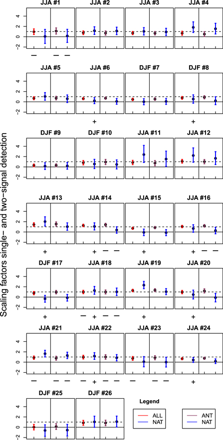
Figure D1. Scaling factors 1- and 2-signal analysis for the 26 regions and for summer temperature. The expected response to the respective forcing (ALL, NAT, ANT) is detected if the best estimate of a scaling factor (dot) and its 5-95% confidence interval (whiskers) are larger than zero. A—symbol underneath a bar indicates that the model internal variability is too large which makes detection results more conservative. A + symbol indicates that the model internal variability is too small.
Download figure:
Standard image High-resolution image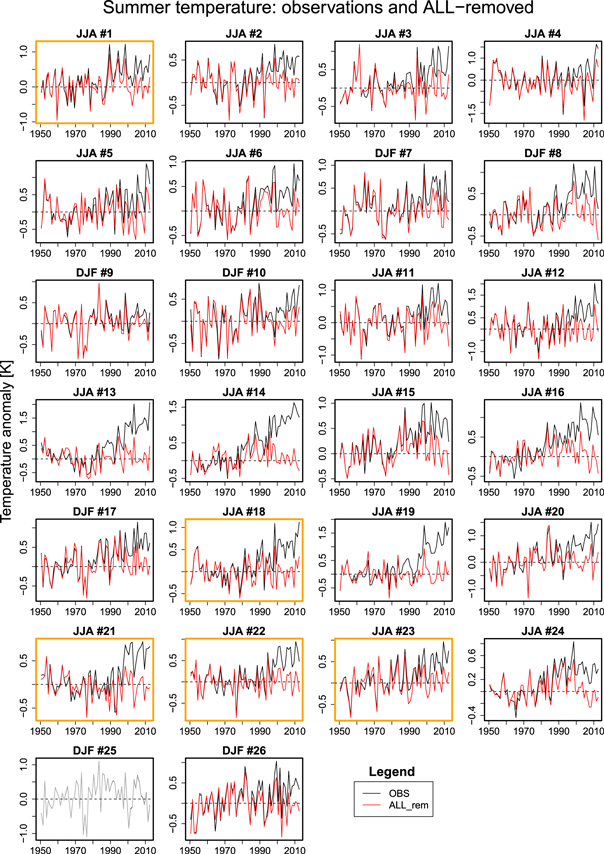
Figure D2. Observations (black) and reconstructed temperatures (red) in summer. The reconstructed temperature is the temperature without the signal from external forcing, and the difference between the red and black line the temperature attributable to external forcing. Grey lines indicate regions where the scaling factor is not distinguishable from zero (see figure D1). Yellow box color denotes regions where the model internal variability is too large.
Download figure:
Standard image High-resolution image
Acknowledgments
We acknowledge the World Climate Research Programme (WCRP)'s Working Group on Coupled Modelling, which is responsible for CMIP, and we thank the climate modelling groups for producing and making available their model output. For CMIP the US Department of Energy's Program for Climate Model Diagnosis and Intercomparison provides coordinating support and led development of software infrastructure in partnership with the Global Organization for Earth System Science Portals. All data have been analyzed using the softwares R version 3.1.0 (R Development Core Team 2008) and IDL version 8.2.3.
Appendix
Appendix A.: List of CMIP5 simulations
Appendix B.: Estimation of FAR uncertainty
To estimate the uncertainty in the FAR (see table B.1 , last two columns), we repeatedly re-sample the 380 chunks of control simulations. The second last column takes into account sampling uncertainty. In the last column, the same procedure is used, but in addition, a sample of scaling factors is drawn for the calculation of the FAR to account for scaling uncertaintyerlaa1c5dt4 . The two different uncertainty estimates were obtained as follows:
Table B.1. Year and temperature anomaly of observed historical maximum temperature, attributable temperature-anomaly, and exceedance probabilities (i.e. probabilities for hot summers) in simulations with external forcing P1 and without forcing (control simulations, P0), as well as the fraction of attributable risk. See also figure 2. The last two columns are different estimates of the uncertainty in FAR: the column 'sampling' presents the 25th, 50th and 75th percentiles of the FAR obtained by re-sampling the 380 control simulations. The resampling was performed 1000 times. The column 'sampling and scaling' includes the uncertainty of the scaling factor.
| Maximum temperature in | Attributable temperature | Exceedance | Fraction of attributable risk (−) | |||||
|---|---|---|---|---|---|---|---|---|
| SREX- | Year with | observations | anomaly | probabilities (%) | 25, 50, 75 p | 25, 50, 75 p | ||
| Region | max. T | T (K) | T (K) | P1 | P0 | FAR | sampling | sampl. and scaling |
| 1 | 1998 | 1.22 | 0.41 | 6.67 | 1.25 | 0.81 | [0.78, 0.81, 0.83] | [0.45, 0.62, 0.70] |
| 2 | 1998 | 0.85 | 0.30 | 2.56 | 0.30 | 0.88 | [0.84, 0.88, 0.91] | [0.00, 0.87, 0.91] |
| 3 | 1962 | 1.19 | 0.00 | 0.77 | 0.30 | 0.61 | [0.35, 0.59, 0.72] | [0.36, 0.60, 0.72] |
| 4 | 2012 | 1.62 | 0.67 | 5.90 | 0.71 | 0.88 | [0.87, 0.89, 0.90] | [0.86, 0.93, 0.95] |
| 5 | 2010 | 1.40 | 0.67 | 5.38 | 0.24 | 0.96 | [0.95, 0.96, 0.97] | [0.84, 0.99, 0.99] |
| 6 | 2010 | 0.96 | 0.50 | 6.67 | 0.24 | 0.96 | [0.96, 0.96, 0.97] | [−Inf,−0.05, 0.30] |
| 7 | 1998 | 1.03 | 0.25 | 4.87 | 1.86 | 0.62 | [0.56, 0.62, 0.67] | [0.40, 0.92, 0.97] |
| 8 | 1998 | 1.20 | 0.40 | 5.90 | 0.83 | 0.86 | [0.84, 0.86, 0.88] | [0.30, 0.81, 0.91] |
| 9 | 1984 | 0.97 | 0.01 | 0.26 | 0.42 | −0.62 | [−Inf,−0.71, 0.01] | [−Inf,−0.84,−0.39] |
| 10 | 1990 | 0.86 | 0.22 | 5.13 | 1.19 | 0.77 | [0.73, 0.77, 0.80] | [0.62, 0.74, 0.78] |
| 11 | 2006 | 1.22 | 0.64 | 5.64 | 0.81 | 0.86 | [0.83, 0.85, 0.87] | [0.53, 0.77, 0.83] |
| 12 | 2010 | 2.03 | 0.94 | 2.82 | 0.22 | 0.92 | [0.91, 0.93, 0.94] | [0.11, 0.61, 0.83] |
| 13 | 2012 | 2.06 | 1.59 | 17.44 | 0.03 | 1.00 | [1.00, 1.00, 1.00] | [−Inf,0.87, 0.89] |
| 14 | 2010 | 1.63 | 1.29 | 17.18 | 0.00 | 1.00 | [1.00, 1.00, 1.00] | [−Inf,−Inf,−Inf] |
| 15 | 2002 | 1.01 | 0.44 | 4.62 | 0.19 | 0.96 | [0.95, 0.96, 0.96] | [0.33, 0.79, 0.98] |
| 16 | 2002 | 1.38 | 0.73 | 3.85 | 0.05 | 0.99 | [0.98, 0.99, 0.99] | [−Inf,−Inf,−Inf] |
| 17 | 2006 | 1.15 | 0.52 | 7.69 | 0.71 | 0.91 | [0.89, 0.91, 0.92] | [0.63, 0.92, 0.95] |
| 18 | 2012 | 1.12 | 0.78 | 15.64 | 0.12 | 0.99 | [0.99, 0.99, 0.99] | [0.66, 0.92, 0.97] |
| 19 | 2010 | 1.90 | 1.43 | 8.97 | 0.00 | 1.00 | [1.00, 1.00, 1.00] | [−Inf,−Inf,−Inf] |
| 20 | 2008 | 1.51 | 0.81 | 8.21 | 0.28 | 0.97 | [0.96, 0.97, 0.97] | [0.60, 0.89, 0.93] |
| 21 | 2008 | 0.90 | 0.73 | 27.95 | 0.63 | 0.98 | [0.97, 0.98, 0.98] | [0.65, 0.95, 0.98] |
| 22 | 2010 | 0.94 | 0.69 | 21.54 | 0.21 | 0.99 | [0.99, 0.99, 0.99] | [0.53, 0.95, 0.98] |
| 23 | 2010 | 0.97 | 0.58 | 17.69 | 2.31 | 0.87 | [0.86, 0.87, 0.88] | [0.78, 0.91, 0.93] |
| 24 | 1998 | 0.83 | 0.29 | 0.51 | 0.13 | 0.75 | [0.51, 0.75, 0.84] | [−Inf,−Inf,0.82] |
| 25 | 1984 | 1.10 | 0.00 | 4.62 | 4.84 | −0.05 | [−0.24,−0.04, 0.08] | [−Inf,−Inf,0.82] |
| 26 | 2000 | 1.03 | 0.40 | 4.62 | 0.61 | 0.87 | [0.84, 0.87, 0.89] | [0.48, 0.76, 0.84] |
B.1. Sampling uncertainty, second last column of table B.1
We re-sample the 380 chunks of the control simulations 1000 times with replace to obtain 1000 times 380 bootstrap samples . We use each bootstrap sample of control chunks to estimate P0 directly from the re-sampled control chunks and P1 from reconstructions produced with the sample of control chunks. We thus calculate

1000 times. We then calculate the interquartile range (25th and 75th percentiles) and the median of these 1000 realizations of the FAR to estimate it is uncertainty. Note that the medians (table B.1) are very close to the single FAR estimate using the original set of control simulations (column 'FAR').
B.2. Sampling and scaling uncertainty, last column of table B.1
We additionally include the uncertainty of the scaling factor by re-sampling the scaling factor 1000 times. We do not know the distribution of the scaling factor obtained from the total least square method (see Ribes et al 2013). However, to roughly approximate the shape of the distribution, we assume a shifted log-normal distribution. The scaling factor (x50) and its 5th (x05) and 95th-percentiles (x95) are obtained from the ROF. If x05 is below zero, we do not calculate the FAR (region 25). If the 5th and 95th-percentile values indicate a right shifted distribution, i.e.  , we first mirror x05 and
  to obtain a left shifted distribution, using the formula
  and
and  . We then calculate the parameters σ (scale parameter) and γ (shift parameter) to minimize the function

with  and with the arbitrary choices of initial values
  and
and  . With the resulting σ and γ values, we generate scaling factors β by selecting values x at random from the uniform distribution on the interval
 ![$\left[{x}_{05}-\tfrac{{x}_{95}-{x}_{05}}{10},{x}_{95}+\tfrac{{x}_{95}-{x}_{05}}{10}\right]$](https://content.cld.iop.org/journals/1748-9326/11/4/044011/revision1/erlaa1c5dieqn8.gif) and then applying the probability integral transform
and then applying the probability integral transform
in order to sample from the shifted log-normal distribution. We then re-transform the resulting values if the original distribution was right shifted. Lastly, we reconstruct P0 and P1 similar to above, but with drawing a different scaling factor for each reconstruction. We calculate 1000 simulations of the FAR with equation (1) and calculate the 25th, 50th and 75th-percentile of the FAR. Table B.1 shows that the interquartile range of the FAR is larger when the uncertainty of the scaling factor is included, as expected.
Appendix C.: FAR for different thresholds
The reader is invited to calculate the fraction of attributable risk for any temperature anomaly at https://summertemperature.shinyapps.io/FAR_App. Note that here, exceedance probabilities are calculated from the entire time series rather than reconstructions for the individual hottest year as done in the main text of the paper.
Appendix D.: Results for individual regions
Table D.1. Median temperature response (K) as estimated by the MMD-A1B-scenario in IPCC (2007), table 11.1. Differences in near-surface temperature between the years 2080–2099 and the years 1980–1999. Note: we excluded SPA, NPA, TNE, IND, CAR and ANTc from this table as they include mostly oceanic areas. Summer is defined as December–February in NAU, SAU, AMZ, SSA, SAF, and as June–August elsewhere.
| Region | Abbrev | Annual | Summer |
| Sahara | SAH | 3.6 | 4.1 |
| Southern Europe and Mediterranean | SEM | 3.5 | 4.1 |
| Central Asia | CAS | 3.7 | 4.1 |
| Central North America | CNA | 3.5 | 4.1 |
| Tibetan Plateau | TIB | 3.8 | 4 |
| Western North America | WNA | 3.4 | 3.8 |
| East Africa | EAF | 3.2 | 3.4 |
| Central America | CAM | 3.2 | 3.4 |
| Eastern North America | ENA | 3.6 | 3.3 |
| West Africa | WAF | 3.3 | 3.2 |
| South Africa | SAF | 3.4 | 3.1 |
| North Australia | NAU | 3 | 3.1 |
| Mediterranean Basin | MED | 2.7 | 3.1 |
| Northern Asia | NAS | 4.3 | 3 |
| East Asia | EAS | 3.3 | 3 |
| Amazonia | AMZ | 3.3 | 3 |
| East Canada, Greenland, Iceland | CGI | 4.3 | 2.8 |
| Northern Europe | NEU | 3.2 | 2.7 |
| South Asia | SAS | 3.3 | 2.7 |
| Sothern South America | SSA | 2.5 | 2.7 |
| South Australia | SAU | 2.6 | 2.7 |
| Southeast Asia | SEA | 2.5 | 2.4 |
| Alaska | ALA | 4.5 | 2.4 |
| Arctic | ARCb | 4.9 | 2.1 |