

Abstract
Changes in vegetation and snow cover may lead to feedbacks to climate through changes in surface albedo and energy fluxes between the land and atmosphere. In addition to these biogeophysical feedbacks, biogeochemical feedbacks associated with changes in carbon (C) storage in the vegetation and soils may also influence climate. Here, using a transient biogeographic model (ALFRESCO) and an ecosystem model (DOS-TEM), we quantified the biogeophysical feedbacks due to changes in vegetation and snow cover across continuous permafrost to non-permafrost ecosystems in Alaska and northwest Canada. We also computed the changes in carbon storage in this region to provide a general assessment of the direction of the biogeochemical feedback. We considered four ecoregions, or Landscape Conservations Cooperatives (LCCs; including the Arctic, North Pacific, Western Alaska, and Northwest Boreal). We examined the 90 year period from 2010 to 2099 using one future emission scenario (A1B), under outputs from two general circulation models (MPI-ECHAM5 and CCCMA-CGCM3.1). We found that changes in snow cover duration, including both the timing of snowmelt in the spring and snow return in the fall, provided the dominant positive biogeophysical feedback to climate across all LCCs, and was greater for the ECHAM (+3.1 W m−2 decade−1 regionally) compared to the CCCMA (+1.3 W m−2 decade−1 regionally) scenario due to an increase in loss of snow cover in the ECHAM scenario. The greatest overall negative feedback to climate from changes in vegetation cover was due to fire in spruce forests in the Northwest Boreal LCC and fire in shrub tundra in the Western LCC (−0.2 to −0.3 W m−2 decade−1). With the larger positive feedbacks associated with reductions in snow cover compared to the smaller negative feedbacks associated with shifts in vegetation, the feedback to climate warming was positive (total feedback of +2.7 W m−2 decade regionally in the ECHAM scenario compared to +0.76 W m−2 decade regionally in the CCCMA scenario). Overall, increases in C storage in the vegetation and soils across the study region would act as a negative feedback to climate. By exploring these feedbacks to climate, we can reach a more integrated understanding of the manner in which climate change may impact interactions between high-latitude ecosystems and the global climate system.
Export citation and abstract BibTeX RIS

Original content from this work may be used under the terms of the Creative Commons Attribution 3.0 licence. Any further distribution of this work must maintain attribution to the author(s) and the title of the work, journal citation and DOI.
Introduction
Although climate is the dominant control on the spatial distribution of vegetation communities, vegetation may in turn feedback to influence the climate. This feedback may be through biophysical factors such as changes in albedo and energy exchange, or biogeochemical factors, such as changes in carbon (C) cycling (Bonan 2008). In particular, it has been well documented that changes in arctic and boreal vegetation can feedback to influence the climate system (Eugster et al 2000, Chapin et al 2005, Euskirchen et al 2010, Shuman et al 2011).
In the boreal and arctic ecosystems of Alaska and northwest Canada, recent vegetation shifts are attributed to dynamics that include treeline migration (latitudinal and elevational), greater shrub cover in the tundra, reduced growth of spruce forests under drought stress, and disturbances such as fire. Each of these shifts may alter the reflectance, energy balance, and carbon cycling of a given ecosystem, resulting in a climate feedback, both regionally (Chapin et al 2005, Euskirchen et al 2009a), or even globally (Betts 2000, Sturm et al 2005). In this region, latitudinal treeline is mapped as the limit of white spruce (Picea glauca) along the south slope of the Brooks Range in Alaska, whereas elevational treeline is mapped for each of the other mountain ranges, ranging from near sea level in western Alaska to approximately 1250 m in the eastern interior (Viereck 1979). In recent decades, both latitudinal and elevational treeline advance in Alaska have been documented (Viereck 1979, Suarez et al 1999, Lloyd 2005). However, studies have also documented reduced growth of both low elevation and treeline white spruce forests due to temperature-induced drought stress (Barber et al 2000, Wilmking et al 2004) or other factors (Brownlee et al 2016). The lower albedo and greater sensible heat flux of forests compared to tundra suggests that northward forest expansion could be a positive biogeophysical feedback to regional warming (de Wit et al 2014), although reduced growth may result in higher albedo, serving as a negative biogeophysical feedback. In concert with changes in treeline, other studies have documented a shrubification of the tundra, including increases in the biomass and abundance of shrubs (Tape et al 2006, Myers-Smith et al 2015). An increase in shrub abundance in the tundra, accompanied by a lower albedo and greater sensible heat flux, may also act as a positive biogeophysical feedback to warming (McFadden and Chapin 1998, Lynch et al 1999, Chapin et al 2000, Euskirchen et al 2009b, Loranty et al 2011, Bonfils et al 2012).
Wildfire is the dominant disturbance regime of the boreal forests in Alaska and northwest Canada, with generally short fire return intervals of 50–150 years (Payette 1992). This creates a mosaic of stand ages across the region, with each forest stand representing a specific post-fire successional stage. Concurrent with hotter, drier conditions, an increased frequency of years with large fires from the 1960s to the 2000s has tripled the area burned in the North American boreal forest region (Duffy et al 2005, Kasischke 2010, Calef et al 2015). This leads to a landscape with a large proportion of young deciduous stands, which have a greater albedo than mature coniferous forests, resulting in a negative biogeophysical feedback to climate warming. Research also suggests that warmer and drier summers in areas covered by tundra may also experience more burning, with climate change projections suggesting that the area burned in tundra will double by the end of this century (Hu et al 2015).
Furthermore, in these high-latitude regions, as temperatures warm, the duration of the snow covered period is reduced, in terms of both an earlier melt in the spring and a later return in the fall (Callaghan et al 2011 and references therein). These decreases in the duration of snow cover result in greater amounts of absorbed solar radiation and a positive feedback to climate warming, in what is commonly known as the snow-albedo feedback loop. Changes in vegetation may interact with changes in snow cover to moderate this snow-albedo feedback loop. For example, as the amount of annual area burned increases, treeless areas, which have a particularly high reflectance when covered with snow, replace forests in the first years following fire, and can thus act to cool the climate (Randerson et al 2006).
In concert with these biogeophysical feedbacks to climate associated with shifts in vegetation and snow cover, we expect biogeochemical feedbacks associated with changes in carbon stored in the soils and vegetation. Permafrost ecosystems store large amounts of soil organic C in the first several meters of the permafrost because decomposition rates are low in these cold, often wet soils (Hugelius et al 2014). Under a warming climate, thawing of additional upper permafrost layers adds soil organic C to the active layer, thereby increasing the pool of decomposable soil organic matter. This pool is labile and could become available for microbial degradation as the active layer continues to deepen (Mueller et al 2015), with fire occurrence potentially adding to this loss of soil C (Mack et al 2011, Turetsky et al 2015). Plant productivity may increase under warmer temperatures thereby sequestering more C (Shaver et al 1991, Natali et al 2012) or it may decrease due to fire and drought stress thereby releasing more C (Beck et al 2011). Storage in soil C pools may also increase with greater inputs from increased plant growth (Gorham 1991, Hobbie 1996). Consequently, although soil C pools may decrease under warmer temperatures through soil organic matter decomposition and combustion during fire, this may be compensated by greater inputs from plants. Thus, the net C balance of these ecosystems will be controlled by the balance between potential changes in plant productivity and release of C from soils.
In previous work, we examined energy feedbacks to climate due to changes in: (1) snow cover at the pan-Arctic scale (Euskirchen et al 2007), (2) both snow cover and vegetation due to shifts in the fire regime across boreal Alaska and northwest Canada (Euskirchen et al 2009a) and, (3) increased shrub growth (but not changes in distribution) and changes in snow cover in arctic Alaska (Euskirchen et al 2009b). Our previous work (Chapin et al 2005, Euskirchen et al 2009a, 2009b) has shown that in arctic and boreal ecosystems, changes in snow cover exert a stronger feedback to warming than shifts in vegetation type. The work presented here builds on these studies by including a more comprehensive suite of the types of vegetation change, including changes in shrub distribution and growth, tundra fires (in addition to boreal fires), advances in treeline, and reduction in forest cover due to drought. We also take a detailed, comparative approach in this study focusing on four distinct ecoregions, or Landscape Conservation Cooperatives (LCCs; Millard et al 2012), in Alaska and western Canada: the Western Alaska LCC, the portion of the Arctic LCC in Alaska and northwest Canada, most of the Northwest Boreal LCC except for some area in the Northwest Territories, and the portion of the North Pacific LCC in Alaska (figure 1(a)). It is important to be able to quantify these feedbacks both spatially and temporally since they occur at differing spatial and temporal resolutions. Specifically, the objectives of this study are to project and quantify biogeophysical feedbacks to climate across these four LCCs for the 90 years from 2010 to 2099 due to: (1) vegetation changes from the abundance of shrubs in the tundra, boreal and tundra fire regimes, latitudinal and elevational treelines, and drought stress, and (2) the timing of snow melt in the spring, snow return in the fall and snow cover duration. We also examine the changes in carbon storage of the vegetation and soils of these ecosystems and provide a general direction of the biogeochemical feedbacks to climate based on these changes in carbon storage. We hypothesized that, even after accounting for additional biogeophysical feedbacks not previously considered, decreases in snow cover would remain the dominant positive feedback to climate warming, and that this positive feedbacks would likely be larger than any negative feedbacks associated with greater early successional forests under a heightened fire regime.
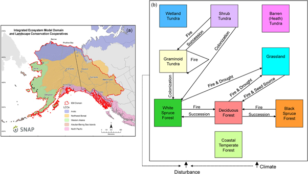
Figure 1. Map of the study area and conceptual diagram of the ALFRESCO model. In (a), the study region in Alaska and northwest Canada depicting the Landscape Conservation Cooperatives (LCCs) that are considered here, including the Arctic, Northwest Boreal, Western Alaska and North Pacific LCCs. Not considered is the Aleutian Bering Sea Islands LCC due to its maritime focus. In (b), a conceptual diagram of the ALFRESCO model illustrating the vegetation types represented in this study and their pathways of change. A one-way arrow indicates that the vegetation transition is one-way. Vegetation types that do not include arrows remain static.
Download figure:
Standard image High-resolution imageMethods
Overview
We performed model simulations for 1900–2100 at a 1 km2 spatial resolution across Alaska and western Canada, and analyzed the outputs for the 90 years between 2010 and 2099. We used a transient landscape-level model of vegetation and fire dynamics, the Alaskan Frame-based Ecosystem Code (ALFRESCO), to estimate the changes in vegetation dynamics associated with: (1) post-fire distribution of the ages of the ecosystems, (2) treeline, and (3) shrubification of the tundra. We used the Terrestrial Ecosystem Model (TEM) to calculate changes in the length of the snow season, incoming solar irradiance and longwave radiation, and changes in vegetation and soil C. We then computed changes in atmospheric heating across the study region due to projected changes in vegetation dynamics, the length of the snow season, and C storage. Below, we provide further details of the study region, the ALFRESCO and TEM models, model input datasets, and calculations of atmospheric heating.
Study region and vegetation map
Our study region focuses on four Landscape Conservation Cooperatives (LCCs; Millard et al 2012) in Alaska and northwest Canada including the Western Alaska LCC and parts of the Arctic, Northwest Boreal, and North Pacific LCCs (figure 1(a)). For simplicity, we refer to these as the Western Alaska, Arctic, Northwest Boreal, and North Pacific LCCs throughout the rest of this paper. These four LCCs correspond to the major ecoregions in Alaska and northwest Canada. To simulate plant growth and treeline dynamics, vegetation composition and distribution, wildfire, and biogeochemistry across the landscape, we relied on a baseline vegetation map of our study region. This map included information from the North American Land Change Monitoring System 2005 dataset (for arctic and subarctic ecosystem types) and the National Land Cover Dataset 2001 (for coastal temperate rainforest ecosystem types), the only two presently available maps with region-wide data for this study.
This vegetation map permitted us to classify the major vegetation types in our study region by LCC, including black and white spruce forest, deciduous forests, maritime coastal temperate forests, heath tundra, shrub tundra, graminoid (tussock) tundra, and wetland (wet sedge) tundra. Although further details of this classification are available in Zhu and McGuire (2016, chapter 2), here we provide an overview of the vegetation composition in each LCC.
The Arctic LCC contains all four types of tundra, with the dominant tundra types relatively evenly distributed between shrub and graminoid tundra, 108 226 km2 and 119 027 km2 respectively (Zhu and McGuire 2016, chapter 2). There were minor components of deciduous forest, and white and black spruce forests, primarily distributed near the southern border of the Arctic LCC, which generally corresponds to latitudinal treeline. The Northwest Boreal LCC consists primarily of deciduous forest (305 051 km2, where the 'deciduous' category consists of both pure deciduous and mixed deciduous-spruce forests), with substantial coverage of pure white spruce forest (120 395 km2) and black spruce forest (88 995 km2), and minor components of all tundra types. The North Pacific LCC is dominated by maritime coastal temperate forest (76 000 km2), and small components of deciduous, white spruce, and black spruce forests. The Western Alaska LCC is relatively evenly dominated by deciduous forest (130 904 km2) and shrub tundra (119 517 km2), with small components of graminoid tundra, and white and black spruce forests. Although we do not explicitly include wetlands, the simulations with TEM (described below) include separate calibrations for three upland and lowland forest types (black spruce, white spruce, and deciduous forests), with lowland vegetation in the black spruce boreal ecosystems generally corresponding to wetlands, while graminoid and wet sedge tundra correspond to wetlands in the tundra ecosystems.
ALFRESCO model
We used a transient, biogeographic model, ALFRESCO (figure 1(b); e.g., Rupp et al 2000, Johnstone et al 2011, Gustine et al 2014, Hewitt et al 2015), to simulate changes in vegetation type due to fire disturbance, natural succession, treeline advance, and shrubification from 2010 to 2100. This model includes the dominant vegetation types of Alaska and northwest Canada as described above, including black spruce forests, white spruce forests, deciduous forests, heath (barren lichen-moss) tundra, shrub tundra, wetland (wet sedge) tundra, graminoid (tussock) tundra, and maritime coastal temperate forests. The heath tundra, wetland tundra, and maritime forests are currently treated as static vegetation states in the model.
The fire module of ALFRESCO uses a cellular automata approach with separate subroutines for cell ignition and spread to simulate annual fire season activity, where additional details on the fire module are provided in Zhu and McGuire (2016, chapter 2). Following a wildfire, burned spruce forest (white or black) transitions into early successional deciduous forest, while burned deciduous forest self-replaces (figure 1(b)). Transitions in tundra are due to succession or colonization and infilling. These tundra transitions are influenced by climate and fire history, which in turn are influenced by proximity to seed source, seedling establishment and growth conditions. For the transition from tundra to forest at treeline, seed dispersal occurs within a 1 km2 neighborhood. White spruce colonization/infilling may occur in both graminoid and shrub tundra with transition rates to spruce forest regulated by climate effects and basal area growth accrual. Drought stress may also influence treeline and vegetation shifts, and is modeled in ALFRESCO based on temperature and precipitation thresholds. Vegetation succession from graminoid to shrub tundra is modeled probabilistically, with a greater likelihood of transition to shrub tundra post-fire. When fires occur in the tundra, shrub tundra transitions to graminoid tundra, and while graminoid tundra is self-replacing (figure 1(b)). Vegetation transitions, defined as at least one shift in vegetation type during the projection period (2010–2099), were calculated as a percent of total area for each of the four LCC subregions. Although a grid cell generally cannot contain a fraction of a vegetation type, there may be an accumulation of white spruce basal area in tundra cells prior to transition to white spruce once the basal areal threshold has been reached. Furthermore, even though ALFRESCO uses an input vegetation map, the model is robust to initialization conditions. The map is used only at the beginning of a 1000 year model spin-up, with random age classes distributed over the landscape, across 200 model simulation replicates. This results in a rapidly converging ratio of vegetation types on the landscape by present time, with additional details provided in Mann et al (2012). The original 'mixed' class was reclassified as deciduous in the initialization vegetation map and the model only considers 'Deciduous or 'Black' or 'White' Spruce. Age is the key factor in determining the transition between 'Deciduous' or 'Black' or 'White' Spruce, and stands that are on the border between age thresholds could be considered 'Mixed', but this is presently not represented in the model. Depending on the age class of a given pixel, the associated probability of burning (cell ignition) is adjusted. The probability of a cell igniting and fire spreading to neighboring cells is also related to temperature and precipitation as well as vegetation type.
TEM with a dynamic organic soil module (DOS-TEM)
We implemented a linear coupling between ALFRESCO and TEM, allowing for the exchange of information between the models to occur in series. Here, the spatially-explicit time series of fire occurrence simulated by ALFRESCO is used to drive the process-based TEM with a Dynamic Organic Soil Module (DOS-TEM; Raich et al 1991, Yi et al 2010, Genet et al 2013). DOS-TEM then simulates the effects of wildfire, warming, and historical logging on carbon pools and aerobic carbon processes. DOS-TEM has been extensively used in arctic and boreal regions, with applications to the soil environment (e.g., Zhung et al 2001, 2003, Yi et al 2010), fire (e.g., Balshi et al 2009), and interactions between fire and carbon storage (Genet et al 2013). Although DOS-TEM has been extensively described in these studies, and most recently in Zhu and McGuire (2016), we briefly describe the model here. DOS-TEM belongs to the TEM family of process-based ecosystem models that are designed to simulate carbon and nitrogen pools of the vegetation and the soil, and carbon and nitrogen fluxes among vegetation, soil, and the atmosphere (Raich et al 1991, McGuire et al 1992). DOS-TEM is comprised of four modules: an environmental module, an ecological module, a disturbance module and a dynamic organic soil module. The environmental module simulates the dynamics of biophysical processes in the soil and the atmosphere, including soil temperature (including permafrost dynamics) and moisture conditions for multiple layers within various soil horizons including moss, fibric and humic organic horizons, and mineral horizons. The ecological module simulates carbon and nitrogen dynamics in the atmosphere, vegetation, and soil, while the dynamic organic soil layer module calculates thickness of the fibric and the humic organic layers, after soil carbon pools are altered by ecological processes (litterfall, decomposition and burial) and fire disturbance. The disturbance module simulates the effects of logging and wildfire on soil and vegetation carbon and nitrogen pools, taking into account the C lost to combustion during wildfires as described in Yuan et al (2012) and Genet et al (2013). For wildfire, the module computes combustion emissions to the atmosphere, the fate of un-combusted C and N pools, and the flux of N from the atmosphere to the soil via biological N fixation in the years following fire. In boreal forest, the amount of soil C combusted during a wildfire is determined using input data on topography, drainage, and vegetation, as well as soil (moisture and temperature) and atmospheric (evapotranspiration) environmental data (Genet et al 2013). In tundra, the rates of combustion are based on estimates from the 2007 Anaktuvuk River Fire (Mack et al 2011).
DOS-TEM takes as inputs information pertaining to climate (monthly mean air temperature, total precipitation, net incoming shortwave radiation and vapor pressure, which is converted to vapor pressure deficit in the environmental module), drainage, soil texture, elevation, and vegetation type. The model is calibrated by vegetation type for rate-limiting parameters represented in the model based on target values of C and N pools and fluxes of representative mature ecosystems. These parameters were 'tuned' until the model reached target values of the main C and N pools and fluxes (Clein et al 2002). For boreal forest communities, an existing set of target values for vegetation and soil carbon and nitrogen pools and fluxes was assembled using data collected in the Bonanza Creek Long Term Ecological Research (LTER) program (Yuan et al 2012). For the tundra communities, we used data collected at the Toolik Field Station (Shaver and Chapin 1991, Van Wijk et al 2003, Sullivan et al 2007, Euskirchen et al 2012, Gough et al 2012, Sistla et al 2013). Finally, for the maritime upland forest, we used data collected from a long-term carbon flux study in the North American Carbon Program (D'Amore et al 2012). The target values for maritime alder shrubland were assembled from Binkley (1982).
As described in Zhu and McGuire (2016, chapter 6), the model has been validated by comparing simulated soil and vegetation carbon stocks with field observations, including soil observations from the National Soil Carbon Network database (Johnson et al 2011) and vegetation biomass estimates from the Arctic LTER database (http://toolik.alaska.edu) for shrub, tussock, wet sedge, and heath tundra as well as forest inventory data collected by the Cooperative Alaska Forest Inventory for upland and lowland black spruce, white spruce and deciduous forest (Malone et al 2009). In terms of the validation of the other modules of DOS-TEM, regional applications of this model in northern high latitudes have included validation at seasonal to century scales for processes related to soil thermal activity (Zhuang et al 2001, 2003a, 2003b), snow cover (Euskirchen et al 2006, 2007), and fire (Balshi et al 2009, Yuan et al 2012, Genet et al 2013).
In this application, the biogeochemical outputs of interest include vegetation C stock estimates, derived from the sum of the above- and belowground living biomass, and soil C stocks. Soil C stocks are composed of carbon stored in the dead woody debris fallen to the ground, moss horizon, organic soil horizons, and mineral soil horizons. We computed regional area-weighted estimates of the vegetation and soil C pools in two ways: (1) by taking into account changes in the area of a given vegetation type, as derived in ALFRESCO, and (2) by assuming the area of each vegetation type remained constant to that in the first decade of the analysis, thereby permitting us to generally understand the impact of changes in vegetation on changes in C pools.
We use the environmental module of DOS-TEM to estimate the changes in the timing of snowmelt, snow return, and the duration of the snow season with methodology previously implemented in Euskirchen et al (2006, 2007, 2009a, 2009b). Snow pack accumulates whenever mean monthly temperature is below −1 °C, and snow melt occurs at or above −1 °C. At elevations of 500 m or less, the model removes the entire snow pack, plus any new snow by the end of the first month with temperatures above −1 °C. At elevations above 500 m, the melting process requires 2 months above −1 °C, with half of the first month's snow pack retained to melt during the second month. We incorporate an algorithm to estimate the date of snowmelt (or snow return) from the monthly estimates of snowpack. This algorithm uses a 'ramp' between monthly temperatures (Euskirchen et al 2007). Linear interpolations of data for monthly air temperature and the month(s) preceding snowmelt (or snow return), the month of snowmelt (or snow return), and the month following snowmelt (or snow return) are performed. For example, to calculate the date of snowmelt when all snow has disappeared by April, approximately 30 points are interpolated between mean monthly March and April air temperature to determine the 15 points for the first half of April and approximately 30 points are interpolated between mean monthly air temperature in April and May to determine the 15 points for the second half of April. The length of the snow-free season is calculated by subtracting the Julian date of snowmelt from the Julian date of snow return. To examine changes in the timing of snowmelt, snow return and snow cover duration between 2010 and 2099, we calculated anomalies based on the mean day of snow melt, snow return and number of days of snow cover duration for the period from 1980 to 2009. We calculate the anomaly for a given decade based on the difference between the day of snowmelt/return or total snow duration for a given decade from 2010 to 2099 minus mean day of snowmelt/return or total duration in the 30 years preceding the prognostic simulations, from 1980 to 2009. As discussed in Euskirchen et al (2006, 2007), the model estimates of the spatial extent and the temporal dynamics of snow cover are in agreement with those of Dye (2002).
Climate data
The baseline period for both the ALFRESCO and TEM simulations was defined as the period from 1950–2009. This period corresponds to the beginning of reliable wildfire observations and statistics for this region (1950) and the end of contemporary downscaled historic climate observations (2009). The projection period was defined as the period from 2010 to 2099. Although the climate inputs to ALFRESCO include air temperature and precipitation, those for TEM include air temperature and precipitation as well as downwelling surface radiation and vapor pressure. Below, we describe the climate datasets and downscaling methods.
Historical (Climate Research Unit—CRU TS 3.1; Harris et al 2014) and projected (CMIP3) output variables of surface temperature (°C), precipitation (mm), and cloudiness (%) were downscaled via the delta method (Hay et al 2000, Hayhoe 2010) using PRISM 1961–1990 2 km resolution climate normals as baseline climate (Daly et al 2008). The delta method was implemented by calculating climate anomalies applied as differences for temperature or quotients for precipitation between monthly future CMIP3 data and calculated CRU climate normals for 1961–1990 (see http://www.snap.uaf.edu for data and details). These coarse resolution anomalies were then interpolated to PRISM spatial resolution via a spline technique, and then added to (temperature, downwelling radiation) or multiplied by (precipitation) the PRISM climate normals. The downscaled climate data were then bias corrected to account for mismatches between the historical and future data, and interpolated to a 1 km2 resolution for modeling purposes.
Monthly surface downwelling shortwave radiation (RSin, MJ m−2 d−1) is calculated for use in TEM and for calculating changes in atmospheric heating. The algorithm takes into account the downscaled cloudiness data (as described above) and the baseline climatology global irradiance (GIRR, monthly, MJ m−2 d−1) to calculate RSin based on an equation from Allen et al (1998) at a monthly time step and 1 km2 spatial scale:

Values of longwave radiation (W m−2) are calculated, including incoming longwave radiation (RLin), outgoing longwave radiation (RLout), and net longwave radiation (RLnet), based on Idso and Jackson (1969), and include a cloud correction factor (Parkinson and Washington 1979). The incoming longwave radiation is calculated as:
This is modified by the cloud correction factor of 1 + cn, where c is the fractional cloud cover value and n is an empirical factor set at 0.275 (Parkinson and Washington 1979). The Stefan–Boltzmann constant (σ) = 5.67 × 10⁻⁸ W m−2 K−4. T is air surface temperature in K.
The outgoing longwave radiation is calculated taking into account the vegetation type and the emissivity values (Ɛ) for the given snow and non-snow covered vegetation type (Geiger et al 2009), in addition to the ground surface temperature (Tg) and the Stefan–Boltzmann law

The net longwave radiation is then calculated by subtracting RLin from RLout. This value is typically negative because the thermal radiative temperature of the atmosphere viewed from the air is cooler than the ground surface temperature (Betts and Ball 1997).
We selected two general circulations models (GCMs) of the best performing subset models for Alaska (Walsh et al 2008), which bound the climate scenarios from most warming and fire activity (the version 5 of the European Center Hamburg Model from the Max Planck Institute ECHAM5; Roeckner et al 2003, 2004) to least warming and more moderate fire activity (the Canadian Center for Climate Modeling General Circulation Model, CCCMA; McFarlane et al 1992, Flato 2005). Our analysis focused on a moderate forcing emission scenario (A1B) for the two GCMs from the Intergovernmental Panel on Climate Change's Special Report on Emission Scenarios (IPCC-SRES; Nakicenovic and Swart 2000). We chose only this one scenario due to the computational complexity and associated long run times with DOS-TEM. The AIB emissions scenario is a conservative choice given that global emissions more closely track the A2 scenario (Peters et al 2012, IPCC 2013), but we did not want to overestimate the amount of land area burned. Further, since we are using just this one emission scenario, we chose to bracket the variability across two bounding GCMs, choosing the CCCMA and ECHAM from a suite of GCMs, after ALFRESCO simulations indicated maximum (ECHAM) and minimum (CCCMA) area burned across the study domain with these two GCMs under the A1B scenario. We analyzed the climate data for the periods from: September–October (the fall shoulder season), November–March (the cold season), April–May (the spring shoulder season), and June–August (summer).
Methodology for computing atmospheric heating
We assessed potential changes in atmospheric heating and feedbacks to climate due to both changes in vegetation following fire, treeline advance, and shrubification and changes in the snow season. Our calculations of atmospheric heating follow the methodology of Chapin et al (2005) and Euskirchen et al (2007, 2009a, 2009b), and are described below.
We first compiled information on albedo (α), latent (LE) and sensible heat (H) fluxes for the dominant vegetation types in our region (table 1). These parameterization sites were eddy covariance sites that collected information on the energy fluxes as well as meteorological variables, including both albedo and snow depth. We distinguished between four distinct periods based on the state of the snow cover as seen in the data: pre-snowmelt (six weeks prior to the final snowmelt, generally from March through mid-April for the boreal ecosystems and from early May to early June for the tundra ecosystems), post-snowmelt (mid-April through late August for the boreal ecosystems and from early June through mid-August for the tundra ecosystems), pre-snow return (six weeks prior to consistently snow covered ground, late August–mid October for the boreal ecosystems and mid-August–mid-September for the tundra ecosystems), and post-snow return (mid-October–early March for the boreal ecosystems and mid-September–early May for the tundra ecosytems).
Table 1. Mean values of energy budget parameters across the dynamic vegetation types modeled in this study. We also include, for comparison, parameters for a boreal thermokarst collapse scar bog and moderate rich fen. Atmospheric heating is given both as a percentage of long- and shortwave net radiation (% of RSnet + RLnet), calculated based on measured heat flux to the atmosphere [sensible (H) plus latent (LE) fluxes], and in MJ m−2 d−1, calculated as in equation (7). Estimated values of albedo (α), H, and LE are obtained from the references. RSin, incoming shortwave radiation; RLin, incoming longwave radiation; RSnet, net shortwave radiation; RLnet, net longwave radiation.
| Vegetation type | Reference | Radiation or energy budget parameter | Pre-snowmelt | Post-snowmelt | Pre-snow return | Post-snow return |
|---|---|---|---|---|---|---|
| Boreal evergreen | Euskirchen et al (2014) | α | 0.40 | 0.09 | 0.12 | 0.41 |
| RSnet + RLnet (% of RSin + RLin) | 7 | 21 | 16 | 6 | ||
| Atmospheric Heating: | ||||||
| (% of RSnet + RLnet) | 38 | 63 | 44 | −6 | ||
| MJ m−2 d−1 | 3.9 | 10.5 | 6.4 | −0.5 | ||
| Boreal early successional deciduous forest | Amiro et al (2006), Liu and Randerson (2008) | α | 0.55 | 0.15 | 0.15 | 0.55 |
| RSnet + RLnet (% of RSin + RLin) | 10 | 17 | 12 | −2 | ||
| Atmospheric Heating: | ||||||
| (% of RSnet + RLnet) | 28 | 68 | 19 | −12 | ||
| MJ m−2 d−1 | 2.1 | 8.2 | 2.5 | −1.4 | ||
| Boreal grass/shrub/early deciduous, 5 yr post-burn | Amiro et al (2006), Liu and Randerson (2008) | α | 0.48 | 0.13 | 0.24 | 0.46 |
| RSnet + RLnet (% of RSin + RLin) | 11 | 26 | 13 | 6 | ||
| Atmospheric Heating: | ||||||
| (% of RSnet + RLnet) | 30 | 57 | 40 | −10 | ||
| MJ m−2 d−1 | 2.4 | 7.0 | 3.3 | −1.1 | ||
| Graminoid tundra | Euskirchen et al (2012) | α | 0.68 | 0.24 | 0.31 | 0.50 |
| RSnet + RLnet (% of RSin + RLin) | 5 | 21 | 17 | −0.1 | ||
| Atmospheric Heating: | ||||||
| (% of RSnet + RLnet) | −1 | 18 | 11 | −3 | ||
| MJ m−2 d−1 | −0.3 | 6.9 | 3.3 | −0.7 | ||
| Barren/lichen/moss (heath) tundra | Euskirchen et al (2012) | α | 0.73 | 0.27 | 0.25 | 0.57 |
| RSnet + RLnet (% of RSin + RLin) | 1 | 18 | 15 | 0 | ||
| Atmospheric Heating: | ||||||
| (% of RSnet + RLnet) | −3 | 16 | 11 | −12 | ||
| MJ m−2 d−1 | −0.7 | 1.9 | 2.8 | −1.5 | ||
| Shrub tundra | Euskirchen et al unpublished data | α | 0.54 | 0.24 | 0.26 | 0.49 |
| RSnet + RLnet (% of RSin + RLin) | 2 | 14 | 20 | 1 | ||
| Atmospheric Heating: | ||||||
| (% of RSnet + RLnet) | 6 | 20 | 12 | 3 | ||
| MJ m−2 d−1 | 1.8 | 7.3 | 3.6 | 0.2 | ||
| Wet sedge tundra | Euskirchen et al (2012) | α | 0.73 | 0.25 | 0.25 | 0.51 |
| RSnet + RLnet (% of RSin + RLin) | 1 | 20 | 16 | 1 | ||
| Atmospheric Heating: | ||||||
| (% of Rsnet + RLnet) | −5 | 60 | 46 | −4 | ||
| MJ m−2 d−1 | −1.0 | 6.2 | 2.9 | −0.9 | ||
| Boreal collapse scar bog | Euskirchen et al (2014) | α | 0.52 | 0.17 | 0.14 | 0.47 |
| RSnet + RLnet (% of RSin + RLin) | 9 | 24 | 16 | 5 | ||
| Atmospheric Heating: | ||||||
| (% of RSnet + RLnet) | −11 | 53 | 36 | −26 | ||
| MJ m−2 d−1 | −0.3 | 6.6 | 2.1 | −1.7 | ||
| Boreal fen | Euskirchen et al (2014) | α | 0.69 | 0.23 | 0.19 | 0.49 |
| RSnet + RLnet (% of RSin + RLin) | 4 | 20 | 14 | 2 | ||
| Atmospheric Heating: | ||||||
| (% of RSnet + RLnet) | −13 | 51 | 34 | −15 | ||
| MJ m−2 d−1 | −0.8 | 6.0 | 1.8 | −1.9 | ||
Based on each period of snow cover and each value of albedo obtained from the field data and RSin obtained from (equation (1)), we calculated outgoing shortwave solar radiation (RSout) as:

Shortwave net radiation (RSnet) is then calculated as the difference between RSin and RSout:

Seasonal atmospheric heating is then computed by multiplying incoming shortwave and longwave radiation by the proportion of incoming shortwave that is absorbed by the land surface times the proportion of net shortwave that is transferred to the atmosphere minus the absorbed and emitted longwave radiation ( ):
):
Note that the ratios in this calculation are key, in that the terms described collapse into ({H + LE} − RLnet), but we have used the ratios to derive H + LE. We estimated changes in atmospheric heating due to changes in the length of the snow season, in terms of both snowmelt in the spring and snow return in the fall. We use DOS-TEM-derived values of RSin and literature-derived values of heat fluxes (table 1) and calculate atmospheric heating for pre- and post-snowmelt based on equation (6). We then compare pre- and post-snowmelt and pre- and post-snow return energy budgets to estimate the changes in snowmelt and snow return on atmospheric heating: {[Daily atmospheric heating post-snowmelt (or pre-snow return)] – [Daily atmospheric heating pre-snowmelt (or post-snow return)]} × [Change in snow cover duration], where the daily atmospheric heating is in units of MJ m−2 d−1 and the change in snow cover duration is in days yr−1. The estimates of heating are then averaged over the length of the snow-free season, as calculated in the water balance model of DOS-TEM. Estimates of atmospheric heating are presented at the decadal time scale in W m−2 based on the mean annual changes in the surface energy flux. Due to the computational complexity and large data files associated with the 1 km2 model simulations in ALFRESCO and DOS-TEM, the vegetation transitions and snow cover are summarized annually across each LCC prior to computing the decadal atmospheric heating feedbacks. Atmospheric heating feedbacks from each LCC are then area weighted by the proportion of the LCC to the total region such that the total regional feedback is the sum of the feedbacks from each LCC.
Results
Climate and snow cover
Across all regions, both GCMs showed trends towards warmer and wetter conditions between 2010 and 2099, although these increases in temperature and precipitation were consistently greater in the ECHAM scenario than the CCCMA scenario (figure 2). The Western Alaska LCC showed the smallest increases in temperature. The Arctic LCC showed the smallest increases in the amount of precipitation in both the ECHAM and CCCMA scenarios, although as a percentage this increase in precipitation could be as large as 70% more precipitation in the future between November and March compared to the historical record during these same months. Increases in precipitation were generally greatest during the cold season from November to March, followed by the fall shoulder season from September to October (figure 2(a)). The fall shoulder season generally showed the greatest warming across each of the four LCCs, followed by the cold season, from November to March (figure 2(c)). There was a general trend towards a decrease in incoming shortwave radiation across both models (figure 2(b)).
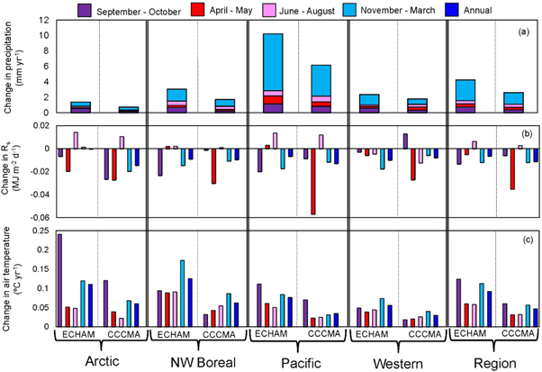
Figure 2. Trends in precipitation, incoming solar radiation, and air temperature across the four Landscape Conservation Cooperatives (Arctic, Northwest Boreal, Northern Pacific, Western Alaska) and regionally, during 2009–2100 based on the outputs from two general circulation models (ECHAM and CCCMA) and one scenario (A1B). Trends are based on the slopes of least-squares linear regression. Under the ECHAM scenario, the following trends are significant at p < 0.0001: precipitation in the fall in the Arctic LCC, incoming solar radiation in the Northwest Boreal LCC, air temperature in the winter in Arctic LCC, air temperature across all seasons in the Northwest Boreal and Western Alaska LCCs, and air temperature in the summer in the Pacific LCC. Under the CCCMA scenario, precipitation, incoming solar radiation, and air temperature in the winter in the Arctic LCC were the only trends significant at p < 0.0001.
Download figure:
Standard image High-resolution imageThese differences in the amount of increase in temperature and precipitation across the two models resulted in differences in changes in the timing of snowmelt, snow return, and the duration of the snow season from 2010 to 2099 (figure 3). The snowmelt anomalies were greatest in the Western Alaska and North Pacific LCCs for the ECHAM scenario (figures 3(c) and (d)). In the Northwest Boreal LCC, the CCCMA scenario generally showed a later snowmelt anomaly from 2010 to 2099 (figure 3(b)). There was a greater change in the timing of snow return anomaly (figures (e)–(h)) compared to the change in the timing of snowmelt, with the change in snow return being smallest for the Northwest Boreal LCC under both the CCCMA and ECHAM scenarios (figure 3(f)). Overall, the change in the duration of the snow season was greatest in the Western Alaska LCC under the ECHAM scenario (an anomaly of 66 days shorter in the last decade, 2090–2099 compared to the mean snow duration from 1980 to 2009; figure 3(l)), with little change in the Northwest Boreal LCC under both the ECHAM and CCCMA scenarios (figure 3(j)).
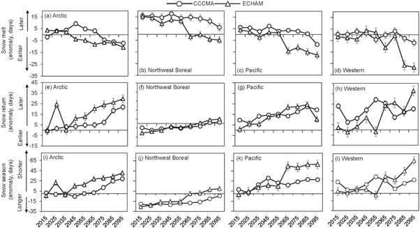
Figure 3. Anomalies of snow melt, snow return, and the duration for the snow season by decade between 2010 and 2099. Anomalies are calculated based on mean date of snow melt, snow return, and total snow cover duration from 1980 to 2009. For snowmelt, a positive anomaly indicates a later day of snow melt and a negative anomaly an earlier day of snowmelt. For snow return and the duration of the snow season, a positive anomaly indicates a later day of snow return or shorter snow cover duration, while a negative anomaly indicates an earlier snow return or longer snow cover duration.
Download figure:
Standard image High-resolution imageVegetation dynamics
Across the region between 2010 and 2099, there was a shift towards a decrease in later successional (≥59 yrs) black and white spruce forests, and corresponding increases in early and mid-successional deciduous forests (0 to 59 yrs; figure 4(a); supplementary appendix 1; figures 1–3). No change was projected in land cover for maritime coastal temperate forest, barren lichen-moss (heath) tundra, or wetland tundra due to the static nature by which ALFRESCO treats these ecosystem types. Consequently, the projected land cover changes were smaller in the North Pacific LCC compared to the other LCCs since the dominant vegetation type in the North Pacific LCC is maritime coastal temperate forest. The decreases in the black and white spruce forests were due to both drought stress and burning. Early, and eventually, mid-successional deciduous forests generally replaced the black and white spruce forests. The loss of graminoid tundra was due to treeline advance, fire, and shrubification. Below, we further describe these vegetation dynamics.
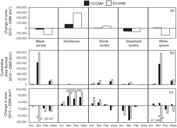
Figure 4. Changes in vegetation (km2) (a), (c) and cumulative area burned (b) from 2010 to 2099 for the CCCMA and ECHAM scenarios. In (a), the overall change between the first decade (2010–2019) and last decade (2090–2099) in a vegetation type is shown, including changes due to shrubification, fire, treeline advance, and drought stress. In (b), the cumulative amount of each vegetation type that burned over the years 2010–2099 is depicted. Panel (c) depicts the overall change in a vegetation regionally, across all four LCCs. 'Arc' = Arctic LCC, 'Bor' = Northwestern Boreal LCC, 'Pac' = Pacific LCC, 'Wes' = Western Alaska LCC.
Download figure:
Standard image High-resolution imageIn the Northwest Boreal LCC, there were similar losses of black and white spruce forest due to fire between the two scenarios (figure 4(b)). However, there was a much larger overall loss of black and white spruce forest in the ECHAM scenario compared to the CCCMA scenario (figure 4(c)), indicating that much of the boreal forest that burned in the CCCMA scenario eventually self-replaced by black or white spruce forest, while the forests in the ECHAM scenario burned more frequently and remained young deciduous forest. Although there was almost no fire in the Pacific LCC (figure 4(b)), there were shifts in vegetation due to natural successional processes, resulting in a decrease in black and white spruce forests and an overall increase in deciduous forests across both the CCCMA and ECHAM scenarios (figure 4(c)).
Across the Arctic, Northwest Boreal, and Western Alaska LCC, the shrub tundra was prone to fire, with greatest burn area in the Northwest Boreal and Western Alaska LCC under the ECHAM scenario (figure 4(b)). However, due to shrubification, these losses in shrub tundra from fire were alleviated in the Arctic and Northwest Boreal LCCs in both the ECHAM and CCCMA scenarios (figure 4(c)), resulting in an overall increase in the area of shrub tundra. This was not the case in the Western Alaska LCC, where the amount of shrubification was less than area of shrub tundra that burned under both the CCCMA and ECHAM scenarios, resulting in an overall loss of shrub tundra.
There were also losses in graminoid tundra across all scenarios due to fire, shrubification and treeline advance, with treeline advance, and the corresponding replacement of graminoid tundra with white spruce forest, accounting for the most of the loss. Regionally, this replacement totaled approximately 31 300 km2 under the ECHAM scenario and 54 100 km2 under the CCCMA scenario. The Northwest Boreal LCC comprised the greatest area where graminoid tundra either burned (figure 4(b)) or was lost due to treeline advance. Here, treeline advance accounted for a loss of approximately 22 000 km2 for the ECHAM scenario and 35 000 km2 for the CCCMA scenario in this LCC.
Vegetation and soil carbon
From 2010 to 2099, vegetation carbon pools increased (figure 5; supplementary appendix 2), even while the area covered by a given vegetation type may have decreased or remained static. There were two exceptions, both in the CCCMA scenario: a slight decrease in the Arctic LCC deciduous forests (−54 g C m−2) and in the black spruce forests of the Western Alaska LCC (−68 g C m−2). Those vegetation types that remained static in cover, barren lichen-moss (heath) tundra, wetland tundra, and coastal temperate forests, all showed increases in vegetation C (supplementary appendix 2). Out of all the vegetation types, the coastal temperate forests in the Pacific LCC showed the greatest increases in vegetation C, by +10 282 g C m−2 in the CCCMA scenario and by +11 746 g C m−2 in the ECHAM scenario, from 2010 to 2099.
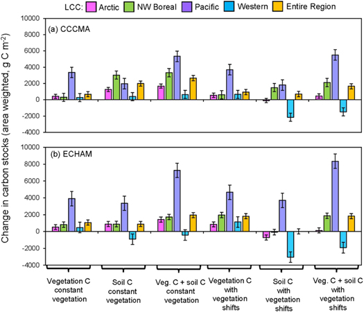
Figure 5. The overall changes in carbon stocks (g C m−2), including vegetation and soil C between the first decade (2010–2019) and last decade (2090–2099) of the period of analysis for the CCCMA scenario (a) and ECHAM scenario (b). The C stocks by LCC are weighted by the proportion of each vegetation type in a given LCC, with vegetation types remaining constant to their proportions of each in the first decade ('constant vegetation') and with vegetation types shifting as modeled in ALFRESCO ('with vegetation shifts') between 2010 and 2099. The regional changes ('Entire Region') are weighted by the proportion of the vegetation type in each LCC and by the proportion of each LCC as a part of the total study region. Changes in vegetation and soil C by vegetation type for the CCCMA and ECHAM scenarios and LCC are provided in supplementary appendix 2.
Download figure:
Standard image High-resolution imageRegionally, soil C also increased from 2010 to 2099, although some vegetation types showed overall decreases in soil C. This included both the CCCMA and ECHAM scenarios for the shrub and heath tundra in the Arctic LCC, the black spruce forests in the Northwest Boreal LCC under the ECHAM scenario, and the deciduous forests in the Pacific LCC under the ECHAM scenario. Notably, in the ECHAM scenario, the Western Alaska LCC showed decreases in soil C across all vegetation types, except for the graminoid tundra and white spruce forests, and in the CCCMA scenario, soil C in this LCC decreased in the black spruce forests and heath tundra.
Regionally, from 2010 to 2099, when considering shifts across the vegetation types, the total change in vegetation and soil C was similar between the two scenarios: +1654 g C m−2 for the CCCMA scenario and +1829 g C m−2 for the ECHAM scenario. If the vegetation remained constant, then the estimates differed by 720 g C m−2, with a change of +2674 g C m−2 in the CCCMA scenario and +1954 g C m−2 in the ECHAM scenario (figure 5).
Atmospheric heating and feedbacks to climate
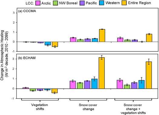
Vegetation shifts resulted in a regional negative feedback to climate of −0.42 to 0.52 W m−2 decade−1 for the ECHAM and CCCMA scenarios, respectively (figure 6). The largest negative feedback occurred in the Western Alaska LCC under the CCCMA scenario (−0.34 W m−2 decade−1; figure 6(a)), and was due to the negative feedback associated with the decrease in shrub tundra following fire, and replacement by graminoid tundra. This negative feedback was large enough to cancel the positive feedback due to changes in snow cover in the Western Alaska LCC under the CCCMA scenario. The second largest negative feedback occurred under the ECHAM scenario in the Northwest Boreal LCC (−0.22 W m−2 decade−1; figure 6(b)). This coincided with the shift from white and black spruce forests to deciduous forests under an intensified fire regime. The only scenario where vegetation shifts resulted in a positive climate feedback was in the Arctic LCC under the ECHAM scenario. This small positive feedback (0.10 W m−2 decade−1; figure 6(b)) was due to both an advancement of treeline and shrubification, and a fire regime of low intensity.
Figure 6. Changes in atmospheric heating (2010–2099, W m−2 decade−1) due to biogeophysical factors (changes in vegetation cover and the snow season duration) for the CCCMA scenario (a) and ECHAM scenario (b). The regional changes ('Entire Region') are weighted by the proportion of the vegetation type in each LCC and by the proportion of each LCC as a part of the total study region.
Download figure:
Standard image High-resolution image
There was an overall positive feedback to atmospheric heating when changes in snow cover were considered in concert with changes in vegetation (figure 6). This positive feedback was larger in the ECHAM scenario across all LCCs (2.7 W m−2 decade−1 over all LCCs) compared to the CCCMA scenario (0.76 W m−2 decade−1 over all LCCs) due to the greater reduction in the length of the snow season in the ECHAM scenario (figure 3). The positive feedback was greatest in the Arctic and Western Alaska LCCs under the ECHAM scenario (∼0.85 W m−2 decade−1 from each LCC; figure 6(b)).
While we did not explicitly estimate the biogeochemical feedbacks due to changes in carbon storage in the vegetation and soils, the increases in C storage indicated that there would be an overall negative feedback to climate in all LCCs except the Western Alaska LCC, where losses in soil C were larger than increases in vegetation C (figure 5). While the biogeophysical feedbacks were small in the Western Alaska LCC (figure 6), large increases in vegetation and soil C in both the CCCMA and ECHAM scenarios by the maritime coastal temperate forests in the North Pacific LCC (figure 5) indicated that this region may be important to consider in terms of climate feedbacks related to changes in C cycling.
Discussion
Overview
Across Alaska and northwest Canada, we simulated changes in vegetation composition, snow cover, and vegetation and soil C stocks under one emissions scenario (A1B) and the climate outputs from two general circulation models, CCCMA and ECHAM. Our simulations occurred at a 1 km2 spatial scale, which is an unprecedented amount of detail for this region. We found that changes in snow cover duration, including both the timing of snowmelt in the spring and snow return in the fall, provided the dominant positive biogeophysical feedback to climate across all LCCs, while changes in vegetation composition generally resulted in negative biogeophysical feedbacks to climate. We expect that there would be a negative biogeochemical feedback to climate since vegetation C increased across all LCCs, and soil C increased across all LCCs except the Arctic LCC under the ECHAM scenario and the Western Alaska LCC under both scenarios. Although other studies have simulated some of these types of feedbacks in high latitudes (e.g., Groisman et al 1994, Betts 2000, Randerson et al 2006, Loranty et al 2011, 2014, de Wit et al 2014), this study provides a comprehensive comparative approach across the ecoregions in Alaska and northwest Canada. Below, we discuss additional details related to these feedbacks and consider other forcing agents that may be important to consider in future studies.
Biogeophysical feedbacks due to changes in vegetation composition
Our results emphasize the importance of considering both tundra and boreal forest wildfire. In the tundra, it was particularly important to consider the burning of shrub tundra. Although studies have suggested that an increase in shrub tundra will act as a positive feedback to climate warming since these shrubs have a lower albedo and greater sensible heat flux than graminoid tundra, previous work has not considered these feedbacks in association with increased burning of shrub tundra (Sturm et al 2005, Euskirchen et al 2009b, Bonfils et al 2012, Zhang et al 2014). Here, we found that while significant amounts of shrub tundra burned in the Arctic, Boreal, and Western Alaska LCCs (figure 4(b)), in the Arctic and Boreal LCCs, there were also increases in the amount of shrub tundra (figure 4(a)) large enough to counteract the greater albedo associated with the burned shrub tundra. In the Western Alaska LCC, there was an overall decrease in shrub tundra, resulting in a negative feedback to climate warming in the CCCMA scenario (figure 6). It is also important to note that shrub height, relative to snow cover thickness, has a key influence over feedbacks to climate, where research shows that shrubs of 0.5 m height having a significantly smaller influence on atmospheric heating than shrubs of 2 m in height (Bonfils et al 2012). Here, our parameterizations of the radiation and energy fluxes for shrub tundra (table 1) were based on a site with shrubs of ∼1 m in height, with shrubs partially exposed all winter. Thus, the positive biogeophysical climate feedbacks associated with shrub expansion would likely be less for the shorter shrubs ≤0.5 m in height, but greater than the taller shrubs >1 m in height.
Wildfire was also important in the Northwest Boreal LCC, with both the CCCMA and ECHAM scenarios indicating large losses of black and white spruce forests that were replaced by young, early successional deciduous forests. This loss of black and white spruce forest was greater in the warmer ECHAM scenario compared to the CCCMA scenario (figure 4(b)). These results support the concept that large expanses of black and white spruce forests in this region may be converted to grasslands or aspen/birch parklands in the coming century under warmer temperatures and an intensified fire regime (Chapin et al 2004, Johnstone et al 2010, Kasischke 2010). The grasslands and deciduous trees (aspen, birch) that establish following fire have a summer and winter albedo that is greater than the coniferous ecosystems (Amiro et al 2006, Liu and Randerson 2008; table 1), thereby resulting in a negative feedback to climate (Beck et al 2011, Rogers et al 2013).
Although fire proved a critical component of this analysis, the biogeophysical climate feedback due to the advance in treeline was negligible. The Northwest Boreal LCC had the greatest increase in the advancement of treeline, but the estimate of this positive feedback was miniscule (≪1 W m−2 for the 90 years from 2010 to 2099). This differs from some other studies in other regions that have found stronger localized positive feedbacks to climate warming associated with changes in treeline (e.g., Pearson et al 2013, deWit et al 2014), and may be due to differences in forest species or faster estimated rates of treeline advance. It is also important to note that in our study area, the Brooks Range provides a natural barrier to treeline expansion (Rupp et al 2001).
Snow cover
It is now well known that changes in snow cover, particularly in spring, can have a strong impact on regional energy budgets due to the considerable amount of incoming solar energy reaching the snow surface (Groisman et al 1994, Déry and Brown 2007, Euskirchen et al 2007). We previously estimated that a pan-Arctic reduction in snow cover of 0.22 day yr−1 during the 1970–2000 period of warming contributed an additional 0.8 W m−2 per decade of energy (Euskirchen et al 2007), a result which is similar to that seen here in the CCCMA scenario (figure 6(a)) for this study region in Alaska and northwest Canada. When comparing climate feedbacks associated with changes in shrub tundra growth to changes in snow cover in arctic Alaska (Euskirchen et al 2009b), we found that greater aboveground biomass from increased shrub NPP produced a decrease in summer albedo, greater regional heat absorption (0.34 ± 0.23 W m−2 decade−1), and a net positive feedback to climate warming. However, this positive feedback was much smaller than the positive feedback due to a shorter snow season (3.3 ± 1.24 W m−2 decade−1; Euskirchen et al 2009b).
Carbon storage
Our simulations with TEM indicated overall increases in carbon storage in the vegetation and soils across the study region, which would result in an estimated negative feedback to climate. Previous simulations with TEM have shown that increases in C storage are associated with the fertilization effect of a rising CO2 concentration (e.g., Hayes et al 2011). Thus, with greater productivity under higher CO2 concentrations, C inputs from litterfall increase, resulting in soil C storage. Historical estimates of simulated soil C stocks and heterotrophic respiration in TEM fall within the range of simulations with other biogeochemistry models across Alaska (Fischer et al 2014). One way to quantify the biogeochemical feedbacks to climate from carbon storage is to employ a fully coupled model of both biogeochemistry and climate that includes the high-level of detail in the arctic and boreal vegetation dynamics we incorporate here, while other methodology can also be implemented (e.g., Frolking et al 2006, Ward et al 2012, Bright et al 2016). It is important to recognize that biogeochemical feedbacks are a global phenomenon, while energy budget feedbacks are predominately local to regional.
The Western Alaska LCC showed loss of soil C, but there is greater uncertainty in this remote region due to a lack of observational data pertaining to climate, vegetation, soils, and disturbance. In future work in the four LCCs considered here, it may be also important to examine the losses of soil C associated directly with regional thawing permafrost and an intensified fire regime. Furthermore, it is important to consider differences in the drier uplands versus the wet lowlands. Simulations with TEM show that the 12% of the study region that is considered lowlands are sources of C, while the uplands are sinks of C (Zhu and McGuire 2016, chapters 6 and 7). We did not include changes in methane (CH4) consumption in our estimate of feedbacks to climate. However, the wetlands in our study region are estimated as increasing sources of CH4, and were the primary reason that the wetlands in the study region were estimated as sources of C (Zhu and McGuire 2016, chapter 7). Consequently, given the smaller proportion of lowlands than uplands, in this present regional assessment, the area remained a C sink, but an expansion of wetlands may result in a greater area that acts as a C source.
Since the version of TEM used here has been developed specifically and optimized for this region, other biogeochemical models with less specific development for our study area may show different results. For example, recent work shows large differences among land surface and biogeochemical models simulated in Arctic Alaska (McGuire et al 2012, Fisher et al 2014). Much uncertainty across models might be associated with differences in the representation of permafrost and to winter respiration (Belshe et al 2013).
Other forcing agents
Other forcing agents that we did not take into account, but which are present in our study area, include thermokarst formation, insect outbreaks, and shifts in the maritime coastal temperate forests. Increases in thermokarst formation (ground subsidence following permafrost thaw) may result in either a negative or positive feedback to climate. In boreal regions, areas that were previously forested, typically by spruce, may become bogs or fens (Jorgenson et al 2001), with a greater albedo and act as a negative biogeophysical feedback to climate. For example, data gathered from a thermokarst collapse scar bog (50 years old) and a moderate rich fen both show year round higher values of albedo and less atmospheric heating compared to spruce and deciduous forests (table 1). As a biogeochemical feedback to climate these thermokarst bogs and fens may sequester either more or less carbon (O'Donnell et al 2012, Jones et al 2013, Euskirchen et al 2014), making their net effect unknown. In arctic regions, typical thermokarst landforms include thermokarst lakes, collapsed pingos, sinkholes, and pits. A key question, both in arctic tundra and boreal forests, is if the number of newly formed thermokarst features would cover a large enough area to induce a significant change in land surface albedo and energy fluxes. Again, a related question is how the creation of these landforms alters the overall carbon storage capacity of the region (Walter Anthony et al 2014, Abbott and Jones 2015), and how this impacts the overall feedback to climate.
Across the forested portions our study area, insect damage can play an important role in tree mortality (FS-R10-FHP 2015). Under warming temperatures in recent decades, a reduction of the beetle life cycle from 2 years to 1 year has in part led to severe spruce beetle outbreaks, with widespread white spruce mortality (Werner et al 2006). Increased disturbance from insect outbreaks will also shift the forest to a younger age classes (Boucher and Mead 2006, Kurz et al 2008) increasing the surface albedo, possibly leading to a negative feedback on atmospheric heating. However, this negative feedback could be counterbalanced by reduced carbon storage capacity in these mature forests with insect outbreaks (Kurz et al 2008).
In future studies that include the North Pacific LCC, it may also be important to include shifts in the maritime coastal temperate forests, which have experienced documented mortality related to climate change (Hennon et al 2012). For example, mortality in yellow-cedar in this region has been related to earlier snowmelt and later freeze-up, where over 200 000 ha of forests have died in the past 100 years (Hennon et al 2006). Moreover, these forests can attract and hold cloud cover, which reflect heat and sunlight (Lawford et al 1996). This potentially strong negative feedback to climate, combined with these forest's carbon storage, are important factors to consider in light of net feedbacks to climate.
Conclusion
A continuing challenge in global change studies is to determine how land surface changes may impact atmospheric heating. Here, we show that even when accounting for a greater number of possible positive feedbacks to climate due to shifts in vegetation than previous studies, including both boreal and tundra fire, an advance of treeline, and increases in the distribution of shrub tundra, changes in snow cover still provided the dominant biogeophysical, land surface positive feedback to atmospheric heating. This positive feedback was partially moderated by an increase in area burned in spruce forests and shrub tundra. It is important to continue to detect changes in vegetation and snow cover, and to combine our knowledge of terrestrial response with that in aquatic environments, including land surface changes caused by a reduction of sea ice, to reach a better understanding of how northern high-latitude ecosystems will influence the climate system.
Acknowledgments
This research was primarily supported by funding from U.S. Geological Survey Alaska Climate Science Center; the Arctic, Northwest Boreal, and Western Alaska Landscape Conservation Cooperatives; and the U.S. Geological Survey Alaska Land Carbon Project. Support was also provided by National Science Foundation through the Bonanza Creek Long Term Ecological Research Program, the Department of Defense's Strategic Environmental Research and Development Program (Project RC-2110), the Department of Energy through the Next-Generation Ecosystem Experiments (NGEE-Arctic), and the EPSCoR Program of the National Science Foundation. Any use of trade, firm, or product names is for descriptive purposes only and does not imply endorsement by the U.S. Government. We thank two anonymous reviews whose comments helped to improve the manuscript.