

Abstract
Worldwide riverine thermal pollution patterns were investigated by combining mean annual heat rejection rates from power plants with once-through cooling systems with the global hydrological-water temperature model variable infiltration capacity (VIC)-RBM. The model simulates both streamflow and water temperature on 0.5° × 0.5° spatial resolution worldwide and by capturing their effect, identifies multiple thermal pollution hotspots. The Mississippi receives the highest total amount of heat emissions (62% and 28% of which come from coal-fuelled and nuclear power plants, respectively) and presents the highest number of instances where the commonly set 3 °C temperature increase limit is equalled or exceeded. The Rhine receives 20% of the thermal emissions compared to the Mississippi (predominantly due to nuclear power plants), but is the thermally most polluted basin in relation to the total flow per watershed, with one third of its total flow experiencing a temperature increase ≥5 °C on average over the year. In other smaller basins in Europe, such as the Weser and the Po, the share of the total streamflow with a temperature increase ≥3 °C goes up to 49% and 81%, respectively, during July–September. As the first global analysis of its kind, this work points towards areas of high riverine thermal pollution, where temporally finer thermal emission data could be coupled with a spatially finer model to better investigate water temperature increase and its effect on aquatic ecosystems.
Export citation and abstract BibTeX RIS

Original content from this work may be used under the terms of the Creative Commons Attribution 3.0 licence. Any further distribution of this work must maintain attribution to the author(s) and the title of the work, journal citation and DOI.
1. Introduction
Riverine ecosystems worldwide face multiple pressures due to human interventions such as dams, channelization, deforestation, and irrigation, to name but a few, as well as a plethora of industrial and agricultural waterborne emissions (Brooker 1985, Meybeck 1989, Bunn and Arthington 2002, Sweeney et al 2004). When combined, physical and chemical stressors can have grave impacts on aquatic ecosystems (Malmqvist and Rundle 2002). One major physical stressor on riverine ecosystems is thermal pollution, a stressor not only problematic in and of itself, but one that can also aggravate the effects of chemical pollution (Heugens et al 2002, Holmstrup et al 2010). Consequently, there is much motivation to identify areas of high thermal pollution.
One of the largest sources of freshwater thermal pollution can be found in the thermoelectric power sector (Hester and Doyle 2011). Power plants stationed along rivers employ two main types of cooling systems, namely once-through and recirculation (tower) cooling. In once-through cooling systems the heat absorbed by the cooling water during the steam cycle is directly rejected back into the river. In a cooling tower setup, on the other hand, most of the absorbed heat is removed via evaporation and dissipated into the atmosphere. The heat contained in the periodic cooling tower blowdown is negligible compared to the heat released in once-through cooling emissions (Stewart et al 2013).
In some rivers, especially those with a series of large thermal emissions sources, the water temperature increase resulting from cooling water emissions can be substantial (Madden et al 2013). Legislative measures in place in the US and in Europe, which impose thresholds for surface water temperature or temperature increase, mean that numerous power stations are forced to restrict their electricity output, often at times of peak demand, and are predicted to do so even more under climate change scenarios (Förster and Lilliestam 2010, van Vliet et al 2012b). Specifically, for the purpose of protecting the aquatic ecosystems, many US states enforce an upper temperature limit of 32 °C for surface water (Madden et al 2013), while in the European Union, water temperatures downstream from the point of discharge should not exceed 1.5 °C and 3 °C above natural temperatures (or 21.5 °C and 28 °C) in salmonid and cyprinid waters, respectively (European Parliament and Council of the European Union 2006).
Previous studies on the impacts of cooling water thermal releases have focused either on the impacts from a single power plant (e.g. Wu et al 2001, Contador 2005, Verones et al 2010) or from multiple plants over large watersheds (e.g. Stewart et al 2013, Pfister and Suh 2015). In a recent study, the cooling systems for the great majority of thermal power plants worldwide were identified (covering 92% of the global thermoelectric power installed capacity), and the thermal emissions for those stations with once-through cooling systems were modelled (Raptis and Pfister 2016). The available data from that work provide a unique opportunity to model power-related freshwater thermal pollution by using these estimates as an input to water temperature models, be they on a small or large geographical scale. The objective of this work is to utilise these heat emission data together with the macroscale hydrological-river temperature model variable infiltration capacity (VIC)-RBM (Liang et al 1994, Yearsley 2012, van Vliet et al 2012b) to obtain the first global view of river temperature increase due to electricity generation.
2. Methods
2.1. Global heat emission dataset
Raptis and Pfister (2016) based their work on the Platts UDI WEPP (World Electric Power Plants Database) version March 2012 (Platts 2012), and analysed the heat emissions from all power plants with once-through freshwater cooling systems worldwide, in terms of the technological, geographical and chronological (age and first year of commercial operation) patterns behind the stations. Vassolo and Döll (2005) used a 12 years older version of the WEPP database (2000) in their study and filled in the missing cooling system information by area-specific statistical and regression analyses. Raptis and Pfister (2016) used Google Earth imagery (Google Inc. 2013) and followed a more laborious procedure similar to that outlined by the USGS for cooling system identification from aerial imagery (Diehl et al 2013). Having covered 92% of the global thermoelectric power installed capacity as reported in the WEPP database, there is confidence that the subset characterised as once-through freshwater and analysed by the authors (amounting to 19% of the global thermoelectric installed capacity) is, to date, the most complete global dataset of power plants employing once-through cooling. The authors characterise the type of freshwater body receiving the emissions, but also provide plant coordinates, determined via individual power plant station information and confirmed via Google Earth imagery (Google Inc. 2013). The thermal emissions were obtained as a direct output of systematically solving the thermodynamic cycle for every generating unit (∼2400 units worldwide) based on the design thermodynamic data in each case, and differentiating between simple, reheat and cogenerative Rankine cycles. Raptis and Pfister (2016) provide maximum heat rejection rates, as well as mean annual ones calculated by multiplying the maximum by mean annual capacity factors. No single source of data that would enable the calculation of monthly capacity factors worldwide was found (the International Energy Agency 2011 provides data that would permit the calculation of monthly capacity factors only for OECD countries on a country and fuel group level). Clearly, monthly thermal emission rates would have been preferable, but for the sake of consistency, mean annual heat rejection rates were used in this work, assumed constant over the months.
For the purpose of investigating the thermal pollution of rivers globally, a subset of power stations rejecting heat into rivers was taken from the dataset available in Raptis and Pfister (2016), excluding emissions into lakes (see section 2.2). A total of 1750 generating units were selected, pertaining to 565 power stations, which account for 12% of the global thermoelectric power installed capacity.
On a country-level, the share of the total thermoelectric power installed capacity represented by the selected power plants varies considerably (figure 1). The United States, China and France are the countries with the highest combined rates of riverine thermal emissions, occupying shares of 26%, 16%, and 12% of the global thermal emission rate respectively, but the power stations with once-through cooling systems along rivers contribute only 17%, 8%, and 25% to the respective national thermoelectric installed capacity (which is dominated by stations employing tower and seawater once-through cooling). In countries where the capacity of the riverine once-through power plants amounts to over 50% of the country-wide thermoelectric installed capacity, the national contribution to the global heat emissions power stations is less than 2%, and the combined contribution sums up to 10% of the global total. While the global and national shares in terms of total thermoelectric capacity occupied by the selected power stations might appear to be small in some cases, considering the completeness of the dataset produced in the work of Raptis and Pfister (2016) and the accuracy of the georeferencing, the dataset used in this study in fact provides the to date most complete quantification of global heat emissions from the thermoelectric sector into rivers.
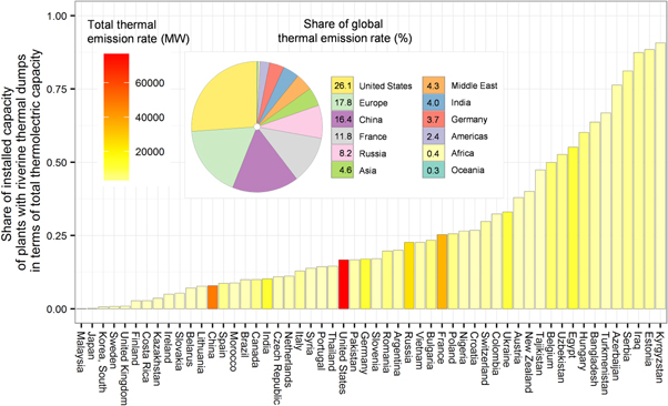
Figure 1. Country-based share of capacity of the riverside power stations with once-through cooling systems selected for this study in terms of the total national thermoelectric power capacity, colour-coded according to the total thermal emission rate resulting from these power plants in each country. The pie chart in the figure inlet shows the fraction these total thermal emissions account for in terms of the global thermal emission rate for the top 12 countries and regions; countries appearing in a category of their own are not included in the regions they belong to (no double counting).
Download figure:
Standard image High-resolution imageFigure 2 shows the spatial distribution of the power plants and the magnitude of the thermal emissions, differentiating between the fuels used in each station (fuel group breakdowns are provided in Raptis and Pfister 2016). Globally, over 46% of the thermal emissions into rivers are due to coal-fuelled power plants and almost one third due to nuclear power plants. According to the analysis carried out by Raptis and Pfister (2016) based on the WEPP database, the majority of power plants with once-through cooling systems are identified in the northern hemisphere and along major rivers. This is in line with the findings of Vassolo and Döll (2005), whose method for populating cooling system data gaps resulted in few power stations being assigned once-through cooling in Asia, Africa, Latin America and Oceania, except for the case of China, where numerous power plants with this type of cooling systems were reported by Raptis and Pfister (2016). Rivers in central-east United States and Europe appear to be heavily burdened by thermal effluents, as do the Nile and the Yangtze. 14 out of the 15 top thermally polluting stations are nuclear power plants, 11 of which are located in Europe, while the greatest thermal emissions from a coal-fuelled power plant come from a station in China.
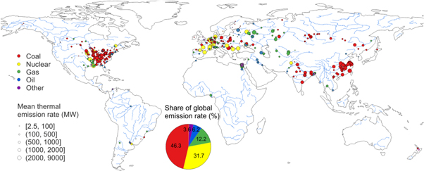
Figure 2. The global distribution of riverside power plants with once-through cooling systems and their thermal emission rate as calculated in Raptis and Pfister (2016). The stations are colour-coded according to their fuel group and the pie chart in the figure inlet presents the combined share of global thermal emission rate per fuel group. Other fuel groups include waste heat, waste, biofuel and geothermal, more details in Raptis and Pfister (2016).
Download figure:
Standard image High-resolution image2.2. Global water temperature impact modelling
VIC-RBM was chosen for this global study assessing the impacts on water temperature of cooling water emissions from the thermoelectric industry, because it is appropriate for large-scale river temperature modelling. It comprises the VIC macro-scale hydrological model (Liang et al 1994) combined with the one-dimensional river temperature model RBM (Yearsley 2009). VIC-RBM is suitable for advection-dominated rivers, it allows for point-sources of heat emissions, and accounts for reservoir impacts on streamflow and water temperature (van Vliet et al 2012a). The modelling framework has previously been applied on a global level and on a 0.5° × 0.5° spatial resolution (van Vliet et al 2013). Water temperature is modelled by solving the one-dimensional heat advection equation in a semi-Lagrangian framework (Yearsley 2009). In this grid-based approach the variables necessary for the solution of the thermal energy budget equation are aggregated per grid cell in nodes that are connected in a river network created by a digital elevation model (Yearsley 2012). The one-dimensional nature of the model means that only emissions into rivers should be considered since the model assumes full mixing in each grid cell. Impacts of thermal stratification of lakes and reservoirs are not included in this version of RBM. For this reason emissions into lakes and reservoirs were excluded in this study, as this would lead to an overestimation of the water temperature increase in the grid cells under question. Therefore, as input to VIC-RBM, riverine emissions were selected from the dataset of Raptis and Pfister (2016).
The VIC-RBM model was applied using the elevation, vegetation and soil characteristics as described in (Nijssen et al 2001), which was later implemented at 0.5° × 0.5° and using the DDM30 routing network (Döll and Lehner 2002) for lateral routing of streamflow. The headwater temperatures (upstream boundary conditions) were estimated using the nonlinear water temperature regression model of (Mohseni et al 1998). Heat emissions are included in RBM as point sources of advected heat as described in (van Vliet et al 2012b). In their study, impacts of heat effluents and reservoirs were included with the aim of improving water temperature simulations in rivers worldwide. Water temperature simulations of RBM were previously evaluated by using observed records of daily water temperature of monitoring stations worldwide from the UN Global Monitoring System (GEMS/Water) combined with other sources for selected river basins (see van Vliet et al (2012a) for details and results of model validation). In this global study, thermal emission rates as calculated by Raptis and Pfister (2016) were aggregated on 0.5° × 0.5° resolution and used as input to VIC-RBM. As an output, the mean monthly river temperature increase above the naturalised water temperature per grid cell was obtained, where the naturalised water temperatures are mean monthly values of water temperature, averaged over the period 1971–2000 (van Vliet et al 2012a).
3. Results
Both globally and in the northern hemisphere the lowest and highest global mean monthly temperature increases were observed in April and October, so these months were selected to showcase the results in figure 3. Large impacts of cooling water emissions on simulated water temperatures were found in many areas in the US and in Europe (figures 3(b)(i–ii) and (c)(i–ii)). In October, when low, if not always minimum annual discharge is observed (see figure S1 in the supplementary information (SI) for examples), a high concentration of heat-rejecting power plants can lead to areas of extensive thermal pollution. In the US, the Mississippi watershed stands out, in particular, the Upper Mississippi, Ohio and Tennessee subbasins (figures 3(b)(i) and (c)(i)). In Europe, the water temperature increase equals or goes above the limit set by the EU (3 °C) over large stretches of the Rhine and Weser watersheds in October (figure 3(c)(ii)), in fact, this temperature increase threshold is met or exceeded over half the year round in these rivers (figure 3(d)(ii)). Moreover, given that the entire area under consideration in Europe is marked as salmonid habitat by the IUCN (2014), an exceedance of 1.5 °C is already considered a problem. Other rivers along which there appears to be considerable increase above the natural background temperature include the Danube and the Po.

Figure 3. For the selected areas with high emission densities: (i) Central-Eastern US and part of Canada, (ii) Europe and North Africa, (iii) China, the following analysis sequence is presented: (a) the mean thermal emission rate aggregated on 0.5° × 0.5° grid cells; the resulting mean monthly river temperature increase above the naturalised water temperature per grid cell in (b) October and (c) April; and (d) a representation of the number of months the 3 °C temperature increase threshold set by EU regulation is equalled or exceeded, scaled by the maximum temperature reached (over the entire year) in the given grid cell. Pink areas mark salmonid habitats (IUCN 2014), which are considered more vulnerable to temperature increase (European Parliament and Council of the European Union 2006).
Download figure:
Standard image High-resolution imageIn some river basins with great amounts of heat emissions the impacts on the river temperature were much smaller, for example in the Nile and the Yangtze (figures 3(b) and (c)). To a large extent this can be attributed to the very high discharge of these rivers at the location of the rejected heat and distinct impacts of large reservoirs, which diminish water temperature rises. Strong effects of evaporative cooling might also have led to smaller water temperature increases in basins with warm atmospheric conditions, such as the Nile, compared to basins in the temperate climate zone.
Figure 4 provides a comprehensive view of the impact of thermal effluents in the most affected basins. Figure 4(a) presents the sum over months and grid cells that the 3 °C temperature increase limit is equalled or exceeded per basin. In essence it shows in absolute terms the cumulative number of instances over the year where significant thermal pollution is observed per basin, while not accounting for the extent of the river section affected. Figure S2(a) in the SI presents the same figure but for all watersheds where an effect on river temperature was observed, that is, with at least a 0.1 °C temperature increase in any given grid cell in any given month. Figure 4(b) (also S2(b)) shows a breakdown in terms of the powering fuel of the total thermal emission rate received in each basin, and figure 4(c) (also S2(c)) presents the distribution in the form of boxplots of the temperature increase over the entire year in the grid cells that were affected in each watershed. Figures 4(a)–(c) cover different aspects of the thermal pollution cause and effect and are completed by figure 4(d) (also S3), which presents the variation over the months of the relative extent of thermal pollution per basin, as a percentage of the total thermally affected flow in each watershed. Specifically, on a monthly scale, the discharge in all unaffected (0 °C temperature increase) and affected (≥0.1 °C temperature increase and defined intervals thereafter) grid cells was summed and related to the total flow of each basin.

Figure 4. For the most affected basins (at least one instance of water temperature increase ≥3 °C in any given grid cell at any given month of the year): (a) the cumulative number of instances (sum over months and grid cells) a 3 °C or higher temperature increase was recorded over the year; (b) the total thermal emission rate colour-coded according to the relevant fuel group; (c) the distribution of recorded temperature increases over the entire year for the grid cells where an impact was observed (i.e. at least one instance of temperature increase) in the form of Tukey boxplots (McGill et al 1978); (d) the monthly variation of portions of the flow unaffected and affected by thermal pollution (according to the defined temperature increase grades) as a fraction of the total watershed flow (the temporal legend is provided in the plot for the Mississippi basin). Figures S2 and S3 present the same plots for the complete range of basins affected (at least one instance of water temperature increase ≥0.1 °C in any given grid cell in any given month).
Download figure:
Standard image High-resolution image
According to the synthesis of figure 4, the Mississippi receives the largest combined thermal emissions, with 62% of them coming from coal-fuelled power plants and 28% coming from nuclear power plant heat effluents. Evidently, due to the scale of the emissions and the basin itself, the absolute number of instances with significant thermal pollution is also large (figure 4(a)). However, in relative terms, the more severely affected portion of the entire Mississippi flow (temperature increase ≥3 °C) never goes beyond 9% of the total flow over the entire year (figure 4(d)). The Rhine receives 20% of the heat emissions the Mississippi receives, almost 3/4 of which come from nuclear power plants, and accumulates many instances of severe thermal pollution over the year, namely over half the number accumulated in the Mississippi (figures 4(a) and (b)). Being a smaller basin, it is therefore more heavily affected than the Mississippi, with 1/3 of its flow experiencing a temperature increase ≥5 °C and only 14% remaining entirely unaffected on average over the year (figure 4(d)). A total of ∼3 GW of heat is released into both the smaller European basins of the Schelde and the Po. However, the thermal pollution intensity patterns vary between the two basins: 46% of the total flow of the Schelde experiences temperature increases ≥3 °C consistently throughout the year. The Po, on the other hand, experiences a surge in the fraction of thermally polluted flow between July–September, when temperatures increase by 3 °C–5 °C and 5 °C–10 °C in 35% and 14% of the total flow, respectively (figures 4(b) and (d)). A high thermal pollution intensity is noted between July–September also in the Weser basin, where over 80% of the total flow is affected by temperature increases ≥3 °C as a result of thermal emissions predominantly due to coal-fuelled power plants (figure 4(b)). These results show that the impact of thermal emissions is of varying magnitude, depending, among others factors, on the geographic conditions and the effect of water management in each basin. In some river basins (in particular basins with large reservoir impacts like the Colorado) heat emissions have very little impacts on simulated water temperature. Figure S3 presents the proportion of thermally unaffected and affected flow for all basins worldwide where an impact (even a small one) was observed, ordered in terms of decreasing share of discharge unaffected by thermal emissions. According to this figure, 3 out of the 5 proportionally most thermally polluted watersheds are located in central Europe, a fact that is troubling given that this area is designated as a salmonid habitat and almost half the proportion of flow in all of these basins over the entire year is affected by temperature increases equal to or exceeding the 1.5 °C temperature increase limit imposed by the EU for the protection of salmonids (European Parliament and Council of the European Union 2006).
4. Discussion
The modelled global thermal pollution must be put into the context of the uncertainties and limitations behind both the heat emissions as well as the model used. As explained in the methods section, in terms of coverage, Raptis and Pfister (2016) obtained a near-complete view of the thermal power plants with once-through freshwater cooling systems, including exact locations, allowing the subset of riverside stations to be identified. However, as the authors point out in their work, the dataset these power plants were identified from, the WEPP database, itself has some weak points (Raptis and Pfister 2016). While for most countries the coverage of the relevant thermoelectric sector is characterised as 'complete' (>95% of facilities), coverage of fossil fuel fuelled power plants with a capacity ≥50 MW in China is characterised as 'comprehensive', that is, including >75% of the facilities in this category (Platts 2012). With coal power plants being the dominant means of thermoelectric generation in China, this under-representation constitutes the major shortcoming with regard to this work. A recent publication gives some insight into what it might actually mean specifically in relation to thermal power plants with once-through cooling systems (Zhang et al 2016). The authors calculate the total installed capacity of thermoelectric power plants with once-through cooling systems in China at 116.1 GW for the year 2011, which is ∼40% higher than the 68.5 GW of the stations identified and analysed for their freshwater heat emissions by Raptis and Pfister (2016). Consequently, there is an underestimation of the thermal emissions and of the modelled river temperature increase in the Chinese basins too.
Electricity production and any ensuing thermal effluents vary greatly over the months as a result of societal demand in response to climatic conditions and more. Reports are plentiful of power stations being forced to regulate their operation to prevent the overheating of freshwater bodies during heat waves (Förster and Lilliestam 2010, Cook et al 2015). The Thermoelectric Power and Thermal Pollution Model (TP2M) is a dynamic model that permits the modelling of power plant adaptation strategies to water temperature and flow variations (Miara and Vörösmarty 2013) and has been applied in studies centred in Northeastern United States (Miara et al 2013, Stewart et al 2013). The use of mean annual heat emission rates as an input to VIC-RBM means that such fluctuations were not captured in this work. This is a clear limitation, as it means that there may well be cases where (a) the river temperature increase has been underestimated, since months of peak electricity output have not been modelled (especially in countries where these coincide with low river flow), or (b) the river temperature increase has been overestimated, due to power plant operational adjustments enforced by local legislation. Nevertheless, the results of this work are still valuable, since they constitute the first concerted effort to model in a consistent way the impact of heat emissions from the thermoelectric power sector on rivers globally, and point to several thermally polluted watersheds.
In terms of the model used, it is likely that the 0.5° × 0.5° grid cell resolution of VIC-RBM was too coarse to capture the effect of thermal emissions in instances where the river discharge is particularly high. This might be the case in the Yangtze basin, for instance, where the total thermal emission rate is the 2nd highest globally, but the modelled river temperature increase appears to be minimal (figures 3(iii) and S2), while in reality the rejected heat might significantly affect certain sections of the river over limited stretches from the point of release, which could be captured by a model with finer spatial resolution.
5. Conclusions
As the first attempt to model the river temperature increase induced by cooling water emissions on a global scale, this work identifies several areas of high concern. The modelled water temperature increases are not trivial if one considers the length covered by a river in a 0.5° × 0.5° grid cell. Large, medium and small river basins are singled out as hot-spots of thermal pollution with varying proportional and temporal patterns. The Mississippi is prominent in terms of absolute occurrences of thermal pollution over its large basin, while smaller European watersheds such as the Rhine, the Weser and the Po see a large fraction of their flow affected by thermal pollution over the entire year, and particularly between July–October. Based on these findings more detailed and localised analyses are recommended for future research, in which riverine thermal pollution patterns are investigated via a hydrological-river temperature model operating on a finer spatial resolution. This would enable the tracing back of the river temperature increase to the responsible power plants and allow for further patterns of thermal pollution to be revealed, in terms of power plant technical characteristics, such as the fuel used, the type of steam cycle employed, the construction year, and more. Such analyses could assist in the compilation of recommendations and strategies for environmental pollution mitigation, particularly if the scope of power plant environmental impacts is broadened, e.g. to include air emissions. Moreover, refining the annual thermal emission rates to a shorter temporal scale (e.g. monthly) before using them in any hydrological-river temperature model, would provide a more realistic pattern of the variation of thermal pollution over the year in many basins and is also recommended for future work. It would also enable the development of adaptation strategies for plant operation to mitigate the effects of thermal emissions during peak months.
It is important to note that the thermal pollution impacts modelled in this work are constrained to those caused by the electricity industry. In urbanised watersheds, heat contained in effluents from wastewater treatment plants can also lead to significant stream temperature increases (Kinouchi et al 2007), and so can the effluent discharges from other industries. As such, the results of this study become even more prominent, since the modelled thermal pollution constitutes the minimum expected anthropogenic perturbation of river temperature through the production of electricity.
It is also worth pointing out that, while the majority of the global heat emissions originate from power plants entering commercial operation during the 1980s or before, and while the use of once-through cooling is generally being phased out in the United States and Europe (Raptis and Pfister 2016), this is not the case everywhere around the globe. The use of once-through cooling has been increasing steadily in China since the 1980s and the current estimation of its share in terms of installed capacity seems even to be underestimated (Raptis and Pfister 2016, Zhang et al 2016). Finally, it is crucial to have current, regionalised estimates of all related impacts, including freshwater thermal pollution, in order to conduct a proper assessment of the trade-off in impacts if and when the once-through cooling systems are replaced by alternative technologies (Sanders 2015, Fricko et al 2016). Among some options, recirculating (tower) cooling overall increases water consumption, dry cooling results in reduced power output (or increased fuel consumption), and once-through cooling with seawater can be problematic when heat dilution at the coast is limited or where reefs are concerned. Quantifying all current impacts, then, is crucial in order to avoid problem shifting, also when switching the power generation technology completely. Ultimately, this work points to hotspots of thermal pollution, where the replacement of old power plants might be prioritised.
Acknowledgments
We would like to thank the anonymous reviewers for their constructive comments and suggestions. We also thank Stefanie Hellweg for her useful suggestions and Eileen Raptis for proofreading the manuscript. Michelle van Vliet was supported by a Veni-grant (project 863.14.008) of NWO Earth and Life Sciences (ALW).