

Abstract
We study the effect of a realistic ice sheet freshwater forcing on sea-level change in the fully coupled Community Earth System Model (CESM) showing not only the effect on the ocean density and dynamics, but also the gravitational response to mass redistribution between ice sheets and the ocean. We compare the 'standard' model simulation (NO-FW) to a simulation with a more realistic ice sheet freshwater forcing (FW) for two different forcing scenario's (RCP2.6 and RCP8.5) for 1850–2100. The effect on the global mean thermosteric sea-level change is small compared to the total thermosteric change, but on a regional scale the ocean steric/dynamic change shows larger differences in the Southern Ocean, the North Atlantic and the Arctic Ocean (locally over 0.1 m). The gravitational fingerprints of the net sea-level contributions of the ice sheets are computed separately, showing a regional pattern with a magnitude that is similar to the difference between the NO-FW and FW simulations of the ocean steric/dynamic pattern. Our results demonstrate the importance of ice sheet mass loss for regional sea-level projections in light of the projected increasing contribution of ice sheets to future sea-level rise.
Export citation and abstract BibTeX RIS

Original content from this work may be used under the terms of the Creative Commons Attribution 3.0 licence. Any further distribution of this work must maintain attribution to the author(s) and the title of the work, journal citation and DOI.
1. Introduction
Sea-level rise is a major topic in climate research, relevant to coastal communities around the world, with an estimated 10% of the population living and working near the coast [1]. The two largest contributors to sea-level rise are ocean thermal expansion and land ice mass loss from the two large ice sheets, Antarctica and Greenland, and glaciers and ice caps [2]. While the primary effect of land ice melt is the addition of mass to the ocean, so-called hosing studies have shown that the runoff of ice sheet freshwater into the ocean may also impact the ocean density and dynamics, and thus also affect (regional) sea-level change [e.g., 3, 4]. Using also high resolution ocean models, the influence of an increased freshwater forcing on for instance the Atlantic Meridional Overturning Circulation (AMOC) can be demonstrated and points to a weakening of the AMOC [e.g., 5]. However, these hosing experiments use much larger freshwater fluxes than the current ice sheet contributions to sea-level change [2].
Climate models from the Coupled Model Intercomparison Project (CMIP) modelling efforts can be used to assess future climate projections, but they generally do not explicitly include ice sheet surface mass balance (SMB) processes [e.g., 6] or ice sheet dynamical processes such as calving. Currently, there are only a few studies that have included interactive land ice freshwater fluxes in a climate model and assessed the impact on sea-level change. Howard et al [7] included both ice sheets and glaciers in the CMIP3-generation [8] HadCM3 model and used the A1B scenario (the Intergovernmental Panel on Climate Change (IPCC) Fourth Assessment Report (AR4) 'business as usual' scenario) to drive the model. In contrast to the results of the hosing studies, Howard et al [7] found that the sea-level change as a result of land ice melt was rather small, with a maximum of 3 cm extra sea-level rise in the North Atlantic above the global mean of 57 cm over the 21st century in their high-end scenario. More recently, Agarwal et al [9] incorporated interactive ice sheet mass change from the IPCC Fifth Assessment Report (AR5) in the CMIP5-generation [10] MPI-ESM model, forced by RCP4.5 and RCP8.5 climate scenarios (Representative Concentration Pathway scenarios [11]). Again, the impact of including ice sheet freshwater fluxes on regional steric sea level was found to be relatively small (up to 2 cm), although in some regions, such as the North Atlantic and Arctic Oceans, values reached up to 4–8 cm by 2100.
Here, we focus on the contribution to (regional) sea-level change of the two large ice sheets, Greenland and Antarctica. Lenaerts et al [12] presented a post-CMIP5 generation model which assimilates a best-estimate of ice sheet freshwater forcing for both ice sheets, but specifically discussed Greenland freshwater runoff for the period 1850–2200, focusing on the impact on the AMOC. They find a decrease of AMOC strength as a result of a warming surface ocean and enhanced Greenland ice sheet freshwater forcing. Here, we use the climate model setup as presented by Lenaerts et al [12, 13] to focus on the effects of changes in historical and future (1850–2100) Greenland and Antarctic ice sheet freshwater forcing on sea level. We compare two different RCP scenarios (RCP2.6 and RCP8.5), to study the impact of ice sheet mass loss both in a mitigation scenario and in a high emission scenario.
An important difference with respect to previous studies that present the effect of ice sheet freshwater forcing on sea level is that this study is the first to simultaneously and consistently show the effect on the ocean dynamical component (changes in ocean density) and on the gravitational component (changes in ocean mass). We will discuss the freshwater forcing (which is defined as the combination of solid ice discharge and liquid surface runoff at the edge of the ice sheet, and excludes incoming mass from precipitation), which can be a result of changes in ice sheet SMB or ice dynamic discharge. We will also discuss the net contribution of ice sheet mass loss to sea-level change, which is the net effect of incoming (e.g. precipitation) and outgoing (i.e. runoff and solid ice discharge) mass on the ice sheets. The direct climate model output allows us to estimate the effect of the ice sheet freshwater forcing on thermosteric and ocean dynamic sea-level (DSL) patterns (hereafter referred to as 'ocean steric/dynamic'). In addition, we use a gravitational sea-level model to show the effect of the redistribution of mass between ice sheets and the ocean on regional sea-level change.
The climate model and the freshwater forcing will be introduced in section 2, along with a description of the sea-level model used to compute the gravitational sea-level pattern. In section 3 we will compare the simulations with a realistic ice sheet freshwater forcing to the simulations that do not have a realistic freshwater forcing, both on a global and a regional scale. Finally, the results will be discussed in relation to previous work, with conclusions drawn in section 4.
2. Methodology
2.1. The Community Earth System Model (CESM)
We use version 1.1.2 of CESM. CESM couples an atmosphere (Community Atmosphere Model, CAM5, [14]), land (Community Land Model, CLM4.5, [15]), sea-ice (CICE, [16]) and ocean model (Parallel Ocean Program, POP2, [17]) interactively. This version of CESM, with a horizontal resolution of ∼1°, is identical to that used in the CESM Large Ensemble [18] and succeeds the version used for CMIP5 [10]. The ocean is initialised by running a control simulation with constant pre-industrial (year 1850) radiative forcing for 1500 years until the upper ocean is in quasi equilibrium with the pre-industrial (1850) climate [18]. Note that the pre-industrial control forcing does not include volcanic forcing, which may lead to an underestimation of the increase in ocean heat content in the historical simulation, when episodic volcanic forcing is introduced [19].
The historical simulation (1850–2005) starts from the final year of the control run, and is followed by the future projections (2005–2100). To drive a transient simulation of CESM, the CMIP5 procedure was followed and CESM was forced with observed greenhouse gas concentrations, aerosols and volcanic activity for the historical period (1850–2005) and with two strongly differing climate change scenarios for the 21st century (2005–2100): a high-mitigation scenario (RCP2.6) and a high-emission scenario (RCP8.5). The CESM variables used in our analysis are ocean temperature (T), ocean salinity (S), sea surface height and ice sheet freshwater forcing, all yearly averaged values.
2.2. Ice sheet freshwater forcing
Lenaerts et al [12, 13] have demonstrated that CESM realistically simulates present-day Greenland and Antarctic ice sheet surface climate, which to a great extent determines the freshwater forcing. However, CESM does not explicitly resolve ice sheet dynamics, and all input mass (i.e. precipitation on the ice sheet) that is not stored in the shallow (1 m w.e.) snowpack is discharged instantaneously to the nearest ocean grid point, as is done in all CMIP5-generation climate models. Essentially this means that CESM assumes the ice sheets to be in long-term mass balance, and the ice sheets are not allowed to lose mass in the form of snowmelt, nor accumulate mass with higher snowfall rates. This is the standard simulation, which we will refer to as the NO-FW simulation.
However, regional climate model results demonstrate that the Greenland snowpack will shrink considerably in the future with higher melt rates [20, 21] and that Antarctic snowfall will be enhanced by higher temperatures [22]. CESM is not capable of representing these future changes and their impact on ice sheet freshwater runoff into the ocean. Therefore, an ice sheet freshwater forcing time series was constructed for both the Antarctic and Greenland ice sheets [12], which was used in the simulation indicated by FW. This freshwater forcing is applied to the CESM ocean grid cells along the ice sheet perimeter and introduced as virtual salinity fluxes to conserve mass in the ocean.
The Greenland freshwater forcing in the FW simulation is derived from a combination of observed solid ice discharge [23] and simulated surface runoff. The solid ice discharge is assumed to remain constant throughout the historical and future period. This is motivated by a combination of factors: observed glacier velocities are showing relatively little inter-annual variability [24], observed ice discharge in 2000–2012 is showing large spatial asynchronousity [23], and the relatively short time period of observations prevents reliable assessment of long-term trends [25]. Icebergs are not modelled explicitly in CESM, but are implicitly included in the solid ice discharge component. The climate model accounts for the release of latent heat as a result of the phase change from solid to liquid freshwater. Solid ice discharge and basal melt fluxes are discharged at the nearest ocean grid point and at the ocean surface.
The Greenland surface runoff for the period 1960–2012 is taken from simulations with the Regional Atmospheric Climate Model RACMO, version 2.1 (RACMO2 hereafter, [21]), forced by ERA-Interim fields at the lateral boundaries. It is assumed that the average runoff in RACMO2 over the period 1960–1989 is representative for the period 1850–1959. Instead of directly using CESM surface water runoff, which poorly resolves Greenland's narrow ablation areas, we use output from RACMO2 to derive a regionally varying relation between mid-tropospheric (500 hPa) summer temperature over Greenland and surface runoff, and apply this to the CESM time series of 500 hPa temperature over Greenland. The method is described in detail in [12].
Unlike in Greenland, surface melt is only marginal on Antarctica and in the FW simulation it is therefore assumed that the projected increase of snowfall on Antarctica [22] will be fully stored in the Antarctic firn. This means we do not consider any SMB-related changes on Antarctica and allow snow mass to accumulate on the ice sheet. We have ignored the potential future runoff from surface melt in coastal regions that is expected to initiate in strong warming scenarios, when the firn pore space is fully depleted [26]. Instead, the most important source of fresh water from the Antarctic ice sheet is ice shelf basal melting at the bottom and calving at the front. To represent this, we apply regionally varying basal mass balance rates from [27] and assume these to be constant throughout the historical period (table 1). In the future, Antarctic solid ice discharge is expected to increase, and therefore we allow a sudden increase of West Antarctic ice loss in 2010–2020 in the Amundsen sea sector along the lines of [28, 29], suggesting rapid ice loss of the Pine Island and Thwaites glaciers, followed by a constant increase in mass loss throughout the remainder of the century (table 1). Given the recent increasing evidence for vulnerability of other sectors of West Antarctica [30] and even East Antarctica [31, 32] to oceanic and atmospheric warming, the Antarctic ice sheet projections used in this study should be treated as conservative estimates. Future work should be directed towards implementing more severe Antarctic mass loss scenarios [e.g. 32] into climate models.
Table 1. Freshwater forcing (Gt yr−1) from the Antarctic ice sheet by sector. Yearly calving flux and basal melt for the period 1850–2010 (constant), yearly total freshwater forcing (=calving flux + basal melt) for 1850–2010 (constant), 2020 and 2100. Based on [27] for 1850–2010, increase of Amundsen Sea freshwater forcing taken from [28, 29], with additional mass loss from Thwaites [29].
| Total FW forcing | |||||||
|---|---|---|---|---|---|---|---|
| West | East | Calving flux (Gt yr−1) | Basal melt (Gt yr−1) | (Gt yr−1) | |||
| Sector | (deg lon) | (deg lon) | (1850–2010) | (1850–2010) | (1850–2010) | (2020) | (2100) |
| Atlantic ocean | 0 | 105 | 204 | 179 | 383 | 383 | 383 |
| Indian ocean | 105 | 170 | 306 | 300 | 606 | 606 | 606 |
| Ross sea | 170 | 215 | 167 | 79 | 246 | 246 | 246 |
| Amundsen sea | 215 | 250 | 232 | 484 | 716 | 846 | 906 |
| Bellinghausen sea | 250 | 305 | 41 | 281 | 322 | 322 | 322 |
| Weddell sea | 305 | 360 | 371 | 131 | 502 | 502 | 502 |
| Total | 0 | 360 | 1321 | 1454 | 2775 | 2905 | 2965 |
2.3. Gravitational sea-level model
Melt water from land ice is not distributed uniformly over the ocean, due to gravitational effects and induced changes in the shape and rotation of the Earth [e.g. 33–35]. The effect of this redistribution of mass is not explicitly modelled in Atmosphere–Ocean Global Circulation Models (AOGCMs) and therefore needs to be added offline. We use a sea-level model to compute sea-level patterns as a result from mass redistribution from the ice sheets to the ocean using a pseudospectral approach [36, 37]. These patterns are computed offline and are added to the sea-level change patterns as a result of wind-, heat- and freshwater-forcing from the climate models, following [38, 39].
3. Influence of interactive freshwater forcing on sea-level change
3.1. Global mean sea level
In the historical period (1850–2005), the freshwater forcing from Greenland in the NO-FW simulation (i.e. direct precipitation runoff) is similar to the forcing in the FW simulation, which is based on the RACMO2 model results (figure 1(a)). There is no significant trend in Greenland freshwater forcing throughout this period in both the FW and NO-FW simulation, as there is no trend in the amount of snowfall over Greenland in the historical period. On average, the freshwater forcing in 1850–2005 is 1050 ± 81 Gt yr−1 (2.90 ± 0.22 mm yr−1 SLE, all uncertainties are  unless otherwise stated, and based on the year-to-year variability of the rates of change) for the NO-FW simulation and 974 ± 48 Gt yr−1 (2.69 ± 0.13 mm yr−1 SLE) in the FW simulation. The small difference is due to the replacement of the CESM precipitation-based runoff with the RACMO2 runoff, which is lower due to refreezing processes in RACMO2, as detailed in [12].
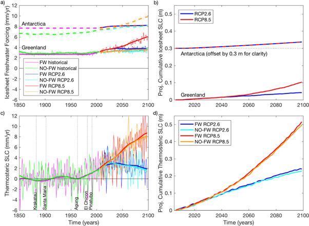
Figure 1. Time series for (a) Greenland and Antarctica freshwater forcing (mm yr−1, yearly and 20 yr running mean), (b) projected cumulative Greenland and Antarctic sea-level contributions (m), (c) thermosteric rates of change (mm yr−1, yearly and 20 yr running mean) and (d) projected cumulative thermosteric sea-level contributions (m). Comparing NO-FW and FW simulations, and historical, RCP2.6 and RCP8.5 scenario's (section 2). In (b), the Greenland cumulative contribution is computed using FW minus NO-FW rates, the Antarctic cumulative contribution uses the change in rate w.r.t. 2005 in the FW simulation (section 3.1).
Download figure:
Standard image High-resolution imageOver the period 2005–2100, the Greenland NO-FW rate is on average 3.25 ± 0.26 mm yr−1 for RCP2.6 and 3.37 ± 0.30 mm yr−1 for RCP8.5 (figure 1(a)). The annual rates of the two FW simulations initially increase more than the NO-FW simulations, but from 2040 onwards the FW-RCP2.6 simulation stabilises (2005–2100 average rate of 3.70 ± 0.31 mm yr−1), while FW-RCP8.5 continues to increase (4.47 ± 0.91 mm yr−1 average rate for 2005–2100). In the RCP2.6 scenario, the global mean temperature only increases with ∼1.5 K between 2005 and 2100, leading to an increase in freshwater forcing in the FW simulation which is approximately equivalent to the increase in the NO-FW simulation that originates from an increase in precipitation and associated runoff. In the RCP8.5 simulation, which projects a ∼4.3 K temperature increase between 2005 and 2100 [18], projected surface runoff increases sharply throughout the 21st century [12], yielding much higher values in the FW simulation than the Greenland freshwater forcing in the NO-FW simulation (figure 1(a)).
The 1850–2005 average contribution of Antarctica (figure 1(a)) is more than double that of Greenland, on average 2414 ± 131 Gt yr−1 (6.67 ± 0.36 mm yr−1) for the NO-FW simulation and 2775 ± 0 Gt yr−1 (7.67 ± 0.00 mm yr−1) in the FW simulation. The lower freshwater forcing in the historical NO-FW simulation is because CESM underestimates snowfall over Antarctica [13], which is not the case in the FW simulation, in which the freshwater forcing is prescribed.
In the 21st century, the average rates increase to 7.75 ± 0.42 mm yr−1 for the NO-FW(RCP2.6) simulation and 8.44 ± 0.88 mm yr−1 for the NO-FW(RCP8.5) simulation. This difference is due to an increase in precipitation as a result of the increased temperature over Antarctica, resulting in more discharge into the ocean. In the FW simulations, the increase in glacial discharge in the Amundsen Sea embayment leads to an additional 0.4 mm yr−1 freshwater forcing, while all the precipitation on Antarctica is assumed to be stored on the ice sheet.
Although all precipitation that falls onto the ice sheets runs off into the ocean in the NO-FW simulations, it does not contribute to long-term (climatic) sea-level change: it is part of the continuous circulation of freshwater between atmosphere, ice sheet and ocean and can therefore only affect sea level in the short term (on seasonal to interannual timescales). However, in the FW simulations the Greenland freshwater forcing does include a potential contribution to long-term sea-level change in addition to the hydrological cycle runoff. We therefore subtract the NO-FW runoff rates from the FW runoff rates and use this to compute the cumulative contribution of Greenland ice sheet to sea-level change (figure 1(b)). This results in a cumulative sea-level contribution of 0.04 m in RCP2.6 (between 2005 and 2100, figure 1(b)), which is within the IPCC AR5 Greenland ice sheet SMB projections 5%–95% range of 0.01–0.07 m [2, table 13.5]. Our RCP8.5 contribution of 0.10 m (between 2005 and 2100) also falls well within the IPCC projected range of 0.03–0.16 m (5%–95%, 1986–2005 versus 2081–2100). In absence of models or data, the future Greenland solid ice discharge is assumed to be constant and therefore will not contribute to sea-level change (see [12] and section 2.2).
In contrast, all of the increase in Antarctic freshwater forcing in the FW simulation is due to an increase in ice dynamic discharge (note that this does not imply that all the freshwater forcing is due to ice dynamic discharge, but only the increase), and it would not be correct to subtract the NO-FW simulations as the increase in precipitation on Antarctica is not expected to run off into the ocean but to refreeze in the snowpack [22]. Therefore, the cumulative sea-level contribution is computed using the differences in rates with respect to the year 2005 in the FW simulation. Since the SMB is assumed constant (see section 2.2), the cumulative sea-level contribution for both scenarios is the same (0.04 m in 2005–2100, figure 1(b)), which is low but within range of the IPCC AR5 value for Antarctic ice sheet dynamics (−0.01–0.16 m, 5%–95%, 1986–2005 versus 2081–2100).
In contrast to the ice sheet contributions, the mean thermosteric sea-level change is small for the initial part of the historical period, and only starts to increase from 1960 onwards (figure 1(c)). The 21st century increase is much larger for the thermosteric contribution than for the ice sheet contributions (figure 1(a)). The NO-FW simulation increases from 0.24 ± 2.06 mm yr−1 in the 20th century to 2.44 ± 1.80 mm yr−1 (RCP2.6) and 5.35 ± 2.71 mm yr−1 (RCP8.5) in the 21st century. The values for the FW simulation are very close: only 0.05 mm yr−1 less for the 20th century and 0.13/0.19 mm yr−1 more for the RCP2.6/RCP8.5 scenarios. This means that the difference in the thermosteric contribution between the NO-FW and FW simulations is relatively small compared to the difference between the scenarios.
Compared to most CMIP5 models presented in IPCC AR5 [2, table 13.5] the thermosteric contribution to sea-level change is quite large (figure 1(d)). For RCP2.6, the cumulative change between 1986 and 2005 and 2081–2100 is 0.24 m (FW) and 0.22 m (NO-FW), which is outside the 0.10–0.18 m 5%–95% range of IPCC AR5. Similarly, for RCP8.5 the cumulative changes of 0.44 m (FW) and 0.43 m (NO-FW) are well outside the 0.21–0.33 m IPCC AR5 range. This indicates that the CESM ocean is very sensitive to radiative forcing variations, compared to other CMIP5 models and observations for the 20th century [40, figure 9.17].
Thermosteric change is driven by many factors, such as atmospheric radiative forcing [41] and temperature, and freshwater forcing from the ice sheets is just one of these factors. The thermosteric contribution is indeed more sensitive to yearly global radiation variations than to ice sheet freshwater forcing changes, leading to much larger variability on a year-to-year basis (figure 1(c)). Some of the negative peaks, for instance, are caused by large volcanic eruptions (figure 1(c), [41]). Another reason for the small difference between NO-FW and FW thermosteric change could be that almost the same amount of freshwater is added to the global ocean, albeit from different locations. We will therefore focus on the regional differences in the next section.
3.2. Regional sea-level contributions
The magnitude of the regional steric/DSL pattern (figures 2(a), (b), (d) and (e)) is mainly determined by the magnitude of the global mean thermosteric change, which appeared not very sensitive to the change in freshwater forcing (figure 1(c) and (d)). The thermosteric change is much more sensitive to the choice of emission scenario, leading to much higher values for RCP8.5 (figures 2(d) and (e)) compared to RCP2.6 (figures 2(a) and (b)). As the more variable regional ocean DSL pattern represents the ocean dynamic deviation from the global mean as a result of atmospheric and oceanic circulation changes and heat and salt redistribution in the ocean, it may therefore be more sensitive to the location of the freshwater forcing than the global mean thermosteric change. For both RCP scenario's, the differences between FW and NO-FW for DSL plus global mean thermosteric change (figures 2(c) and (f)) are slightly positive in most places (0–0.05 m), since in the FW simulation the thermosteric change is slightly larger than in the NO-FW simulation. However, both in the RCP2.6 and the RCP8.5 scenario there are larger differences in the Southern Ocean, Arctic Ocean and in the North Atlantic (locally over 0.1 m). In the Southern Ocean, this seems to be at least partly driven by the location where the freshwater is discharged into the ocean: in the NO-FW simulation most runoff is from Antarctica as the precipitation is allowed to run off, while in the FW simulation most runoff comes from Greenland, as the Antarctic precipitation is assumed to refreeze in the snowpack. In the North Atlantic, the difference may be a result of enhanced weakening of the AMOC due to more realistic Greenland freshwater forcing [12].
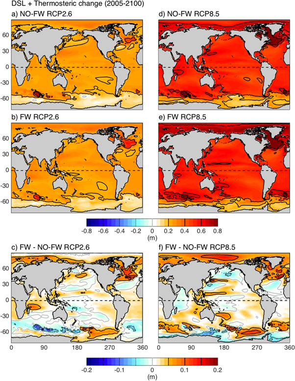
Figure 2. The thermosteric plus ocean dynamic effect of freshwater forcing (cumulative m over 2005–2100) of the Greenland and Antarctic Ice Sheets in NO-FW (a)/(d) and FW (b)/(e) simulations and the difference between FW and NO-FW (c)/(f); for RCP2.6 (left column) and RCP8.5 (right column).
Download figure:
Standard image High-resolution imageIn addition to the ocean steric/dynamic change discussed in the previous paragraph, there is also an effect on sea level as a result of the redistribution of mass between the ice sheet and the ocean. These mass-driven sea-level change patterns are computed with the gravitational sea-level model (section 2.3), using the cumulative ice sheet contributions presented in the previous section (figure 1(b)). The sea-level patterns as a result of ice sheet mass change are so-called 'gravitational fingerprints'. These fingerprints show a loss (gain) of gravitational attraction at the source of the mass loss (gain), leading to a sea-level fall (rise) close to the source. The largest sea-level rise as a consequence of the gravitational pull/push due to ice sheet mass loss is found in the 'far field', where values can be up to approximately 120%–130% of the global mean value.
The regional patterns as a result of the redistribution of mass from the ice sheets to the ocean (figure 3) show this gravitational effect clearly, with sea-level fall close to the ice sheets and most sea-level rise in the West Pacific Ocean for the Greenland contribution (figures 3(a) and (b)) and in the Pacific and Atlantic Oceans for Antarctic ice mass changes (figure 3(c)).

Figure 3. The projected sea-level contributions of the (a)/(b) Greenland, (c) Antarctic and (d)/(e) combined Greenland + Antarctic ice sheets (cumulative m over 2005–2100), under RCP2.6 (left column) and RCP8.5 (right column). The Greenland cumulative contribution is computed using FW minus NO-FW rates, the Antarctic cumulative contribution uses the change in rate w.r.t. 2005 in the FW simulation.
Download figure:
Standard image High-resolution image
As there is a larger projected Greenland ice sheet contribution to sea level in the RCP8.5 scenario than in the RCP2.6 scenario (figure 1(b)), the far-field maxima are also larger for the RCP8.5 scenario (figures 3(a) and (b)). The fast gradient changes in the direct vicinity of the Greenland ice sheet are an artefact of the construction of the sea-level contribution, due to the subtraction of the NO-FW simulation from the FW simulation. Whereas in total the ice sheet loses more mass than it gains in this construction (leading to an overall contribution to sea-level rise), locally the forcing in the NO-FW simulation may be positive where the forcing in the FW simulation is zero, creating artificial mass gain in some grid points. This artefact only affects the sea-level change in the vicinity of the ice sheets, which should therefore be treated with caution.
For Antarctica (figure 3(c)), the largest contribution to sea-level change is from the Amundsen Sea sector (table 1), which translates into the largest sea-level fall in that area. The sea-level change gradually becomes more positive for larger distances to the ice sheet, with maxima at ∼90° radial distance, which is in the Indian Ocean, the North Pacific and the North Atlantic.
The combined mass signal of Greenland and Antarctica shows how both ice sheets contribute equally in the RCP2.6 scenario (figure 3(d)), while Greenland mass loss is more dominant in the RCP8.5 scenario (figure 3(e)). Given the location of the ice sheets (near the poles), the combined far-field maxima roughly occur between 30°N and 30°S. The location depends on the distribution of the mass loss: the larger Greenland contribution in the RCP8.5 pushes the maxima slightly more southward (figure 3(e)) than in the RCP2.6 scenario where the contributions are more equal (figure 3(d)).
Although the steric/DSL changes (figure 2) are larger than the projected mass-driven contribution from the ice sheets (figure 3), the latter does make up a quarter (RCP8.5) to a third (RCP2.6) of the projected sea-level change [2]. As the increase in ocean heat content in this particular climate model is large compared to the CMIP5 models [40, figure 9.17], these ratios may become even larger for climate models that have smaller thermosteric contributions.
4. Discussion and conclusion
Ice sheets are an important and integral part of the climate system, but are not routinely included in climate models in an integrated way. Here, we studied the effect on sea-level change when a realistic ice sheet freshwater forcing is included in the fully coupled CESM. We examined both the effect on the ocean dynamics and on the gravitational, mass-driven sea-level change. We did not include the effect of a freshwater forcing resulting from glacier and ice cap mass loss outside the large ice sheets, but note that the magnitude of this contribution is significant (accounting for approximately 25% of present-day sea-level rise [2]) and should therefore be included in total sea-level projections [e.g., 2, 38, 39, 42]. We compared a 'standard' model simulation (NO-FW simulation) to a simulation with a more realistic ice sheet freshwater forcing (FW simulation) for two different forcing scenario's (RCP2.6 and RCP8.5). Our analysis focused on the 21st century, which is when the ice sheet contribution to sea-level change is projected to increase more than in the 20th century, when the ice sheets are generally assumed to be in mass balance.
We found that the effect of a realistic freshwater forcing on the thermosteric sea-level change is small (∼2 cm for 2005–2100) compared to the total thermosteric change (ranging from 22 cm for RCP2.6 NO-FW to 52 cm for the RCP8.5 FW simulation) and the scenario-driven difference (∼28 cm between RCP2.6 and RCP8.5). Part of the reason for the small difference in the global mean between NO-FW and FW is that the amount of freshwater flowing into the ocean is similar, but with different causes, i.e. precipitation runoff versus ice dynamic discharge, and in different locations, i.e. Greenland versus Antarctica. Another reason is that the global thermosteric change is driven by many processes and only for a small part determined by the amount of freshwater flowing from the ice sheets into the oceans. However, looking at the regional pattern rather than the global mean, we find that the ocean steric/DSL pattern shows larger differences in some regions in response to more realistic freshwater forcing from the ice sheets (locally over 0.1 m between 2005 and 2100, larger values in the RCP8.5 scenario), such as the Southern Ocean, the North Atlantic and the Arctic Ocean. The increasing ice sheet freshwater forcing will not only impact ocean warming, but also the strength of the AMOC. In a previous study [12] it has been shown that the AMOC strength decreases as a result of a larger Greenland ice sheet freshwater forcing. It is therefore important to include interactive ice sheets in future climate model simulations. There are plans to do this in the forthcoming Ice Sheet Model Intercomparison Project under the CMIP6 framework (ISMIP6, http://climate-cryosphere.org/activities/targeted/ismip6).
Our results agree with the findings of Agarwal et al [9], who included the IPCC AR5 time series for Greenland and Antarctic mass change in the Max Planck Institute for Meteorologys Earth System Model for RCP4.5 and RCP8.5 scenarios. When ice sheet freshwater sources are integrated into the climate model, they find differences of mostly up to 2 cm in regional steric sea-level change by 2100, but with larger values in the North Atlantic and the Arctic Ocean. Another study by Howard et al [7] included not only ice sheets but also glaciers in the HadCM3 model, driven by the SRES-A1B scenario, and compared a mid-range to a high-range mass loss scenario. Even though the freshwater flux is larger, given that glaciers are included as well as the ice sheets, they find smaller differences (between including and excluding mass-loss in the climate model) than in the present study, of up to 3 cm in the North Atlantic. This may be caused by their use of the A1B scenario, which has less warming than the RCP8.5 scenario over the 21st century. Interestingly, they find a negative difference between the two simulations in the Arctic Ocean, in contrast to a positive value in this study and the study by Agarwal et al [9], which may be due to their addition of freshwater from glacier mass loss, but could also be related to the use of a different climate model. In conclusion, the patterns and magnitudes of the differences between the NO-FW and FW simulations seem to agree quite well with other studies that have performed similar analyses using different climate models, despite using different methodologies, freshwater sources and climate scenarios. This suggests that the response of the climate models to a plausible 21st century land ice freshwater forcing is small, and robustly so, across different climate models.
The projected regional sea-level contributions as a result of the redistribution of mass from the ice sheets to the oceans due to climate change was computed separately. This showed how the amount of mass loss on the Greenland and Antarctic ice sheets determined the locations of the maxima in the regional sea-level change pattern. Although the ice sheet mass loss is currently smaller than the thermosteric sea-level change or the glacier contribution to sea-level rise [2, table 13.1], it is equal to or larger than the difference in the ocean steric/dynamic contribution as a result of the ice sheet freshwater forcing (figures 3(d) and (e) versus figures 2(c) and (f)). As the ice sheets are expected to increasingly contribute to sea-level rise in the next century and beyond (albeit with large uncertainty as to how much exactly, [2]), the gravitational pattern as a result of ice sheet mass loss will become increasingly important for regional sea-level change projections.
Acknowledgments
We thank two anonymous reviewers and J Church and X Zhang for comments on earlier versions of the manuscript. We thank Miren Vizcaino (Delft University of Technology) and Leo van Kampenhout (Utrecht University) for performing the CESM simulations. AS was supported by a CSIRO Office of the Chief Executive Fellowship and the NWO-Netherlands Polar Program. JTML was supported by Utrecht University through its strategic theme Sustainability, sub-theme Water, Climate & Ecosystems, and the Innovational Research Incentives Scheme of NWO. Part of this work was carried out under the programme of the Netherlands Earth System Science Centre (NESSC), financially supported by the Ministry of Education, Culture and Science (OCW). CESM model output and freshwater forcing time series are available upon request (jtmlenaerts@gmail.com).