

Abstract
The impacts of unpredictable ecological perturbations are often assessed via measurements of environmental change only after the event has occurred. Temporal series of satellite images provide a cost-effective way to gather information before ecological perturbations occur. However, in previous studies, the disturbances have neither been always centred in time in the series of the focal environmental variable nor has the relevance of the temporal coverage been explicitly tested through factorial designs. In this study, we manipulated the temporal coverage and the position of the disturbance event in the temporal series to examine whether and how the assessment is affected. Specifically, we tested the effect of the Prestige oil spill on monthly sea chlorophyll concentration and net primary productivity along the north-western Spanish coast. We designed planned comparisons through factorial analyses to test two alternative hypotheses: (1) the spill has negative consequences on phytoplankton activity and/or abundance due to physiological constraints or (2) it has positive consequences on phytoplankton abundance as a result of changes in biotic interactions. The relevance of the statistical effects was critically dependent on the temporal coverage and the position of the spill event in the temporal series. Short periods (three years) were insufficient to cover the range of variability even if the disturbance was centred in the time series. Similarly, results from longer time series (up to eight years) in which the event was temporally biased (at the beginning of the time series) also differed from those that were centred in the entire time window. Temporal series for the study of ecological impacts should be as long as necessary to encompass the temporal variability of the study systems (up to nine years in our study case), and the disturbance event should be centred in the time series to reduce potential spurious effects of temporal autocorrelation. However, our results revealed that each one of these requirements alone was not sufficient to encompass all of the natural variability, and thus both requirements should be met. For impact assessments we encourage the use of unbiased satellite data series to complement in situ measurements.
Export citation and abstract BibTeX RIS

Content from this work may be used under the terms of the Creative Commons Attribution 3.0 licence. Any further distribution of this work must maintain attribution to the author(s) and the title of the work, journal citation and DOI.
1. Introduction
How organisms and ecosystems respond to natural and anthropogenic perturbations, such as fires, floods, outbreaks, species invasions, habitat fragmentation, nuclear accidents or spills, is a central issue in environmental monitoring and conservation biology (Pascual and Guichard 2005, Banks et al 2013, Simberloff et al 2013). Stability, tolerance and the recovery capacity of key species or communities in the face of ecological perturbations can provide insights not only for future management but can also help to answer fundamental questions about ecosystem functioning. Our partial knowledge on many aspects of nature together with our limitations to perform experimental manipulations in entire ecosystems at different scales necessarily limits our assessments of such responses. A major challenge is disentangling the real impacts of ecological perturbations from the natural variability in a system. There are a number of environmental fluctuations that may be confounded with perturbation effects when natural variation parallels the pattern predicted by the impact, thereby leading to a false rejection of a true null hypothesis (false positive or type error I).
A partial solution to overcome limitations inherent to correlational approaches used to assess the effects of ecological perturbation is to include data from both before and after the perturbation in the analyses (Underwood 1994). After a perturbation event, temporal variation in biotic factors may differ from the variation that was observed before the perturbation occurred. Depending on the time window, these differences may be due to a transition toward the previous equilibrium or because the system has already reached a new stable state with a different regimen of associated fluctuations (sensu Gunderson 2000, Scheffer et al 2001). Thus, information on variation in biotic factors that existed before the perturbation event provides a valuable reference. However, when and where drastic perturbation events, such as fires or spills, will occur is unpredictable; therefore, in situ measurements of biotic factors before the events are often scarce. Even when restricting analyses to a temporal window after the perturbation, in situ measurements may be prohibitive in terms of the time and resources needed. To complicate matters, the length of the time series needed to cover the entire range of variation of the target variable is unknown, thereby increasing the risk of operating with temporally biased data.
Satellite data are being increasingly applied to examine environmental changes, such as those of primary productivity, which may reflect ecological responses (Pettorelli et al 2014, Rose et al 2015). Time series of satellite images have the potential to document variation in biotic factors both before and after an unpredicted ecological perturbation has occurred and for longer and unbiased temporal periods, in a cost-effective manner. Remotely sensed data provide an opportunity to take a more accurate look at how temporal bias might affect conclusions regarding the potential impacts of an ecological perturbation. However, while there are many ecological studies emphasizing that spatial biases often affect the results of models (Zvuloni et al 2008, Rocchini et al 2011, Hijmans 2012), studies that have examined the potential spurious effects arising from temporal bias in data are comparatively rare (Desaules 2012).
The aim of this study was to examine whether and how temporal bias could affect conclusions made on the impact of an unpredictable ecological perturbation at the most basal level of the trophic chain. As a case study, we tested the potential effects of the accident of the single-hulled oil tanker 'Prestige' on sea chlorophyll concentration along the north-western Spanish coast (Galicia) using satellite derived data. The spill commenced on 13 November 2002, 52 km from the coast (42.8 N, −9.8 W), when one of the ship's tanks burst during a storm (González et al 2006). Following the burst, the ship erratically navigated around the area due to pressures from the Spanish, French and Portuguese authorities preventing the ship from approaching the coast. When the ship was 250 km from the coast on the 19 November 2002, it split in half and sank. Three consecutive slicks arrived at the Galician coast on the 13–19 November 2002, 19 November–10 December 2002, and 6 December 2002–9 January 2003. The Prestige oil spill is considered to be one of the major disasters in a marine ecosystem (CEDRE 2009, Penela-Arenaz et al 2009). Oil residues have been detected in the coast even nine years after the accident (Bernabeu et al 2013). More details on the movements of the Prestige, and on the spatial and temporal coverage of the slicks inside and outside of the study area can be found in González et al (2006), and Penela-Arenaz et al (2009).
We selected this study case for several reasons. (1) The Prestige oil spill negatively affected a number of diverse taxonomic groups (Penela-Arenaz et al 2009, Barros et al 2014), but how the spill specifically affected various taxa was not always clear. (2) Previous research on the effect of the Prestige oil spill on chlorophyll concentration reported conflicting results, depending on the framework used for analyses (experimental manipulations versus correlational time series, (e.g. Varela et al 2006, González et al 2009, Moreno et al 2013)), the scale (micro, meso and macro scales (e.g. Varela et al 2006, González et al 2009, 2013)) and temporal coverage (Varela et al 2006, Lee and Kim 2008, Moreno et al 2013). None of the previous studies on time series of satellite-derived primary productivity used a temporal frame in which the temporal position of the spill event was centred, hence obtaining a comparable set of temporal variation before and after the spill was lacking. (3) The Prestige oil spill has been considered to be a complex case due to the high natural variability in phytoplankton activity in the area (e.g., Varela et al 2006). Therefore, to account for other sources of natural variability we also tested for potential effects on net primary productivity (NPP) as a function of chlorophyll concentration and fluctuations of sea surface temperature within temporal series. Thus, we integrated chlorophyll concentration (potentially affected by the spill) and the effect of temperature fluctuations (not necessarily associated with the spill) on chlorophyll efficiency to derive realistic estimates of primary productivity (NPP, see methods). Satellite-derived primary productivity is a valuable indicator of the status of the base of the trophic chain (Irigoien et al 2013).
We have deliberately manipulated the length in years of time series and the temporal position of the spill in the series. Thus, we make use of satellite data to emulate limitations of a type of temporal bias more typically associated with in situ measured data. Previous research on the impacts of oil spills on phytoplankton has supported either negative impacts, via physiological constraints, or indirect positive impacts mediated through changes in the trophic interactions (Johansson et al 1980, Gin et al 2001, González et al 2009 and references therein). Therefore, for each relevant month we performed factorial analyses with planned comparisons designed to test for either positive or negative effects (see methods). This was possible by conducting comparisons of monthly values between the year of the spill and those years with the highest and lowest mean values within the target time series to assess the positive and negative effect predictions, respectively.
2. Methods
2.1. Data sources
Monthly sea chlorophyll a concentrations (mg m–3) for the period 1997–2010 for all available months were obtained from satellite images from the SeaWIFS instrument at the NASA Ocean Color Web and processed with the SeaDas software package (http://oceancolor.gsfc.nasa.gov/). Monthly sea NPP (mg carbon/m2/day) was obtained from a vertically generalized production model (VGPM), which varies as a function of chlorophyll concentration, maximum production potential, day length and euphotic depth (Behrenfeld and Falkowski 1997). For this study, we analysed NPP estimates from the Eppley-VGPM algorithm, obtained also from the Ocean Colour Web. The Eppley algorithm differs from other VGPM-NPP calculations in that the maximum potential is an exponential function of sea surface temperature used to account for photoacclimation (Eppley 1972, Morel 1991). We used the SeaWIFS data because it is closest to meeting our requirement that the Prestige accident (November 2002) be centred in the temporal series. For our analyses we used data on monthly chlorophyll a concentration and NNP at 9 km cell resolution along the north-western Spanish coast (Galicia, figure 1). Oil-spill impacts are usually higher in coastal zones because of higher levels of biodiversity and because concentrations of hydrocarbons are often higher than offshore, including the Prestige oil spill (González et al 2006; reviewed in Penela-Arenaz et al 2009).
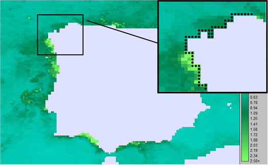
Figure 1. Location of the Galician coast on the Iberian Peninsula. Black dots denote the coverage of the analyses. Increasing average sea chlorophyll concentrations (mg m–3) of March 2002 are represented from cyan to light green at 9 km of resolution.
Download figure:
Standard image High-resolution image2.2. Factorial design and analyses
For the design of our analysis, we considered as reference those months that fulfilled two criteria: (1) when the spill was present in the study area in 2002–2003 (November, December and January), and (2) the months of the lowest (winter) and highest (blooms) values of chlorophyll concentration or NPP across the entire period (1997–2010), encompassing thus the entire seasonal variation. The months corresponding to these minimum values through the entire period coincided with those selected by the first criterion (figure 2). Figure 2(a) shows a bimodal distribution of the mean chlorophyll concentration across months for the entire period. Maximums of spring and summer blooms in the study area correspond to March and September, respectively. Figure 2(b) shows a unimodal distribution of our estimation of NPP, with a maximum that corresponded to August. Therefore, subsequent comparisons were focused on November 2002, December 2002 and January 2003 as relevant months for either chlorophyll concentration and NPP. Comparisons were also focused on March 2003 and September 2003 for chlorophyll and August 2003 for NPP in order to encompass the seasonal variation.
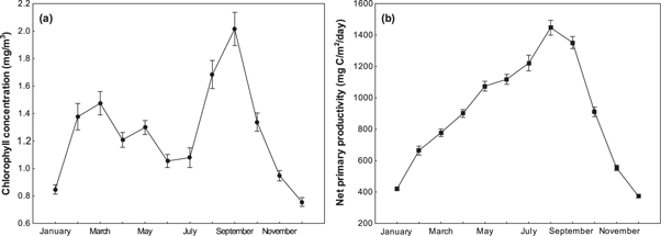
Figure 2. The mean ± standard error of monthly variation for (a) sea chlorophyll concentrations and (b) net primary productivity in a 9 km band along the Galician coast. Time coverage was from 1997 to 2010.
Download figure:
Standard image High-resolution imageFor our analyses, we performed planned comparisons (Quinn and Keough 2002) to explicitly test our target hypotheses (see below). With this procedure we reduced the number of comparisons (among all possible combinations), while also reducing the probability of incorrectly rejecting a true null hypothesis. Thus, each relevant month/year (November 2002, December 2002, January 2003, March 2003 and August or September 2003) was compared with the same month of other years. Comparisons were planned for three different temporal windows that varied in length and/or in the position of the spill event in the time series: (1) contiguous years (three contiguous years where the focus month/year was centred in the time series); (2) after the spill (from the spill event to the end of the series, encompassing an average of six years); and (3) the entire period (depending on the month, 12–14 and 10–12 years for chlorophyll and NPP, respectively). Thus, the contiguous-years period, despite being centred, might be too short to encompass all of the natural variability. The after-spill period emulates a case where the temporal range is longer, but measurements were taken only after the ecological disturbance has occurred, and hence it is strongly biased toward the start of the time series far from the centre. Our use of the entire period enhances the probability of encompassing the entire temporal fluctuation, and the disturbance event is reasonably centred in the series.
We performed general linear models (GLM) separately for each temporal window, where the dependent variable was the chlorophyll concentration or the NPP in a given relevant month and the within-subject factor was one of the temporal windows for the same month. We planned different comparisons depending on the temporal window and the hypothesis being tested. For the contiguous-years period, the factor consisted of three levels (years before, during, and after spill for the same month), and we specified a single contrast for each month to test whether the year of the spill differed significantly from the other two years (just before and after the spill). Thus, this specific contrast design for the contiguous-years period served to test the two hypotheses (both negative and positive effects). For the other two periods (after-spill and entire periods), the factor had two levels that varied with respect to the hypothesis. To test for a negative impact of the spill so that it cannot be confounded with natural variation, the values of the year of the spill should be lower than those of the year that showed minimum mean values in the series. Thus, the contrast was between the year of the spill and the year with the lowest value in the focus time window. For instance, to test for a negative effect in November, we compared 2002 versus 2008 when testing the after-spill period (because 2008 shows the minimum value for this period) and 2002 versus 2000 when considering the entire period, (because 2000 shows the minimum value for the entire period, figure 3(a)). We applied the opposite reasoning to test for a positive impact, where the contrast was between the year of the spill and the year with the highest value in the time window.
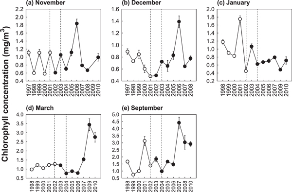
Figure 3. Temporal series of sea chlorophyll concentration (mean ± standard error, N = 52–54) along the Galician coast for (a) November, (b) December, (c) January, (d) March, and (e) September. Black dots denote time after the slicks, and white dots denote time before the slicks. Dashed frames represent the shorter period of analyses corresponding to a three year interval centred in the year/month closest to the spill.
Download figure:
Standard image High-resolution image
We followed two procedures to account for potential non-independence of data. Because this study concerns longitudinal data (i.e. repeated measures for each grid-cell along several years within each month), we performed repeated measures GLMs (Quinn and Keough 2002) in our factorial design, which allows site variability, including spatial autocorrelation, to be accounted for. Finally, to check our repeated measures analyses indeed accounted for spatial autocorrelation in the study area, we examined whether the inclusion of relevant spatial filters (Rangel et al 2006) in our analyses modified our results. We considered as relevant spatial filters those whose Moran's I > 0.5 and their residuals (from the regression with the dependent variable) minimized Moran's I (Bini et al 2009).
3. Results
3.1. Negative-effect hypothesis
For November and December 2002, when major slicks occurred in the study area, comparisons of monthly chlorophyll concentration significantly matched the prediction of negative effects depending on the period of analyses. For November 2002 monthly chlorophyll concentration was significantly lower than in 2001 and 2003 (contiguous years period, within dashed lines in figure 3(a) and table 1). For December 2002 chlorophyll concentration was significantly lower than the minimum within the period after the spill (2007 for December, figure 3(b) and table 1). However, when considering all of the available variation (the entire period), there were no significant differences for either November or December (table 1, figures 3(a) and (b)). For the remaining months (January, March and September), significant effects were inconsistent with the negative-effect hypothesis (table 1, figures 3(c)–(e)). However, at this step, planned pairwise comparisons were designed to test negative effects and hence did not account for the variability of the maximum values (positive-effect hypothesis) for the after-spill and entire periods.
Table 1. Comparisons of monthly sea chlorophyll concentration among years considering three different time windows within the temporal series. Planned comparisons for the periods after the spill and the entire period were designed to test the hypothesis of negative effects (see methods).
| Period of analysis | ||||
|---|---|---|---|---|
| Month during or after the spill | Contiguous years | After the spill | Entire period (1997–2010) | Explanation |
| November 2002 | F1,52 = 88.85 p < 0.0001* | F1,52 = 1.86 p = 0.18 | F1,51 = 0.90 p = 0.35 | Significant effects in the predicted direction only for the contiguous years (figure 3(a)) |
| December 2002 | F1,52 = 47.35 p < 0.0001 | F1,53 = 33.62 p < 0.0001* | F1,53 = 0.32 p = 0.58 | Significant effects in the predicted direction only for the period after the spill (figure 3(b)) |
| January 2003 | F1,53 = 122.14 p < 0.0001 | F1,51 = 62.14 p < 0.0001 | F1,53 = 146.85 p < 0.0001 | Inconsistent with the prediction of a negative effect (figure 3(c)) |
| March 2003 | F1,53 = 4.72 p = 0.034 | F1,53 = 31.37 p < 0.0001 | F1,53 = 31.37 p < 0.0001 | Inconsistent with the prediction of a negative effect (figure 3(d)) |
| September 2003 | F1,53 = 16.74 p = 0.00 015 | F1,53 = 22.05 p < 0.0001 | F1,53 = 34.93 p < 0.0001 | Inconsistent with the prediction of a negative effect (figure 3(e)) |
Note: asterisk denotes significance only when the direction of the effect was consistent with a positive impact.
When considering inter-annual variation in temperature in our analyses (our estimates of NPP), there were significant effects in the predicted direction only for the shortest period both for November and December (contiguous years period, supplementary data table S1, figures S1(a) and (b)). For the remaining months (January and August), significant effects were inconsistent with the negative-effect hypothesis (supplementary data table S1, figures S1(c) and (d)). However, in this case planned pairwise comparisons were designed to test negative effects and hence did not account for the variability of maximum values (positive-effect hypothesis) for the after-spill and entire periods.
3.2. Positive-effect hypothesis
Monthly chlorophyll concentration in January 2003 was significantly higher than in 2002 and 2004 (contiguous years period, within dashed lines in figure 3(c) and table 1) and also significantly higher than in the year of highest value within the period after the spill (table 2, 2007 in figure 3(c)). However, when considering all of the available variation (the entire period), chlorophyll concentration before the spill in January 2001 was significantly higher (table 2 and figure 3(c)). Chlorophyll concentration in September 2003 was significantly higher than in 2002 and 2004 (contiguous years period, table 1, within dashed lines in figure 3(e)), but the effects on the other periods were inconsistent with the positive-effect hypothesis (table 2 and figure 3(e)). For November and December 2002, significant effects were inconsistent with the positive-effect hypothesis for all of the periods.
Table 2. Comparisons of monthly sea chlorophyll concentration among years considering two different time windows within the temporal series. Planned comparisons were designed to test the hypothesis of positive effects (see methods).
| Period of analysis | |||
|---|---|---|---|
| Month during or after the spill | After the spill | Entire period (1997–2010) | Explanation |
| November 2002 | F1,52 = 121.78 p < 0.0001 | F1,52 = 121.78 p < 0.0001 | Inconsistent with the prediction of a positive effect (figure 3(a)) |
| December 2002 | F1,53 = 100.69 p < 0.0001 | F1,53 = 100.69 p < 0.0001 | Inconsistent with the prediction of a positive effect (figure 3(b)) |
| January 2003 | F1,53 = 34.00 p < 0.0001* | F1,52 = 190.70 p < 0.0001 | Significant effects in the predicted direction only for the partial periods: contiguos years (table 1) and after the spill (figure 3(c)) |
| March 2003 | F1,53 = 47.28 p < 0.0001 | F1,53 = 47.28 p < 0.0001 | Inconsistent with the prediction of a positive effect (figure 3(d)) |
| September 2003 | F1,53 = 47.03 p < 0.0001 | F1,53 = 47.03 p < 0.0001 | Significant effects in the predicted direction only for the contiguos years (table 1 and figure 3(e)) |
Note: asterisk denotes significance only when the direction of the effect was consistent with a positive impact.
NPP in January 2003 showed the same pattern of significance as chlorophyll concentration, which was consistent with the positive-effect hypothesis only for the partial periods (contiguous years and after-spill periods, supplementary data table S1, table S2, figure S1(c)). November and December also showed the same pattern of significance for NPP as the chlorophyll concentration (supplementary data table S1, table S2, figures S1(a) and (b)). For the NPP of August, there was no significant difference for the contiguous years period (supplementary data table S1, figure S1(d)), and the effects for the other periods were inconsistent with the positive-effect hypothesis (supplementary data table S2, figure S1(d)). The inclusion of relevant spatial filters in our planned comparisons did not affect the significance (or non-significance) of any effect, for chlorophyll concentration nor NPP (results not shown).
4. Discussion
In this study, satellite imagery allowed us to manipulate the length and bias of temporal series using a correlational approach to examine how these manipulations might affect conclusions on the potential impacts of an ecological perturbation. As an example, we analysed changes of monthly phytoplankton activity and production around the Prestige oil spill because both reflect the availability of resources at the base of the trophic chain and hence are potentially important indicators of ecosystem function and services. We planned comparisons to test either hypotheses of negative or positive effects for short but centred time series, for intermediate and uncentred series, and for longer and centred series, while controlling for site idiosyncrasies and taking into account spatial autocorrelation.
When the analyses were restricted to the shortest but equidistantly centred period (three contiguous years), potential effects on monthly chlorophyll concentration and NPP were always significant except for August. For the intermediate-duration but completely uncentred period, when the time coverage was extended to all available years after the spill, effects were still significantly relevant for months in which the slicks were present in the study area (December and January). After the spill, mean values for December 2002 were always lower than the following years (black symbols in figure 3(b); supplementary data figure S1(b)), which provides support for the negative-effect hypothesis. Thus, at this step a negative impact of the spill on phytoplankton activity is statistically supported for December. However, the effect lost significance for the target hypotheses when the entire period (the longest centred period) was considered.
A common pitfall in correlative analyses of temporal series that are not long enough to encompass the entire range of temporal variability is that temporal autocorrelation can lead to misinterpretations. This is the case for our comparison of chlorophyll concentration in December among years after the spill (black dots in figure 3(b)), in which the spill event is strongly skewed to the beginning of the series. That is, there was an increase in December values that could be explained by a subsequent recovery of chlorophyll concentration after a negative impact from 2002 to 2006. However, when examining a longer time window, the observed pattern strongly suggests that these changes should be due to other sources of variation at larger temporal scales. In fact, there is a U-shaped pattern that significantly fits to a quadratic polynomial at a 10-year temporal scale (1997–2006 in figure 3(b); F1,529 = 119.79, p < 0.0001), showing that there was a decrease in December values before the spill occurred (from 1997 to minimum values in 2001). Thus, the analyses of the after-spill period showed that the lowest values for December in the year of the spill (table 1) merely reflect the right arm of the quadratic temporal pattern from 2002 to 2006 (figure 3(b)).
If we take the most skewed time window of our study (after the spill) and move it backward one or two years and then we apply our analysis design, it would be enough to encompass the total range of variability for November and December. Thus, the comparisons are no longer significant for chlorophyll concentration (November: F1,51 = 0.90, p = 0.35, figure 3(a); December: F1,53 = 0.32, p = 0.58, figure 3(b)). That is, just slightly moving the spill event toward the centre of the time series reduced bias in such a way that potentially spurious effects disappeared. Ideally, the disturbance event should be centred in the time series and be equidistant from the beginning and the end of the temporal series of analyses. The more centred the disturbance event in the time series of the focus environmental predictor, the higher the chance to reduce noise due to other causes that are different from the analysed disturbance, such as temporal autocorrelation. However, our results also showed that this property is not enough to account for the entire range of environmental variability when the time series is too short, as was the case of the contiguous-years period despite the fact that the spill event was perfectly centred in the time series.
If we had relied only on the partial periods (contiguous years or after the spill), our results would be compatible with mechanistic hypotheses of either negative (November and December) or positive impacts (January). Previous experiments that have aimed to replicate the potential effects of the Prestige spill at the microcosm level showed that there is a direct negative effect of oil on photosynthetic efficiency via physiological constraints, which was then followed by indirect positive effects on phytoplankton biomass mediated through biotic interactions (González et al 2009). For this experiment, the potential underlying mechanisms for the negative effect was that slicks reduced the penetration of light into the water, and/or that the accumulation of certain oil compounds in the thylakoid membranes of cells interfered with electron transport and photosynthesis. On the other hand, the subsequent indirect positive effects may be due to changes in the trophic interactions within the plankton community, which were attributed to a decrease in the abundance and/or activity of consumers independent of photosynthetic efficiency (González et al 2009 and references therein). Similarly, the reported increase in phytoplankton biomass and productivity after the oil spill from the tanker Tsesis was explained by the decline in grazing zooplankton populations (Johansson et al 1980). Without our results from the entire time series, it would be tempting to suggest that the aforementioned sequential mechanisms explain negative impacts in December and then positive effects in January. However, mesocosm experiments simulating the same spill revealed that the effects were of much lower magnitude than those previously recorded at the microcosm level (González et al 2013). Moreover, in situ studies on the effects of the Prestige spill concluded that changes in plankton did not show any clear pattern (Varela et al 2006).
Previous studies on the impact of the Prestige spill on chlorophyll concentrations restricted their analyses to post-incident time series data (Moreno et al 2013), pre-incident data (Varela et al 2006) or only to three years at the same spatial resolution (Lee and Kim 2008). For these first two studies, the spill event was not centred in the time series, and the third one used data with different spatial resolutions. Interestingly, of these studies, only the one that analysed the shortest period claimed the existence of a detectable impact (Lee and Kim 2008). This is consistent with our results, where only the shortest period yielded significant effects in the predicted direction, which strongly suggests that the inability to study the entire variation will lead to type I error.
Studies reporting no effect of slicks on plankton around the globe usually give three different non-mutually exclusive explanations. Potential effects may depend on the seasons, the toxicity level of spills may be compound-dependent and may not affect all plankton species equally, while others have argued that the natural variability is so high and complex that the studied effects may be overridden (Lee et al 2009, Penela-Arenaz et al 2009, Neuparth et al 2012). More relevant to the Prestige incident, non-detectable effects have been associated with high natural fluctuations and to the fact that the spill was coincident with the period of lowest phytoplankton activity (Varela et al 2006, Penela-Arenaz et al 2009 and figure 2). For instance, chlorophyll anomalies have been demonstrated to significantly parallel temperature oscillations in the Northern Hemisphere at both monthly and annual temporal scales, although the exact mechanism remains elusive (Raitsos et al 2014). Regardless of whether temperature plays a direct role or is acting as a surrogate predictor, its inclusion in our models was not sufficient to control for all of the natural variation. Despite taking sea surface temperature into account as a source of variation in NPP, the effect of the oil spill on chlorophyll anomalies was still within the range of variation of the entire time series. Another important source of inter-annual variation in the N-NW Spanish coast in winter is the Iberian Poleward (Navidad) Current (Le Hénaff et al 2011), whose unusual strength in 2002/2003 years conditioned slick movements (García-Soto 2004, Acuña et al 2008). Another potential cause for the lack of effects at our scale and resolution may be the heavy nature of the fuel oil, which is associated with low solubility and a low capacity for dispersion in seawater (González et al 2006).
Finally, no effect beyond the natural variation at our spatio-temporal scale and resolution (9 km and the month, respectively) does not necessarily imply that there were no effects at other spatial and temporal scales and resolutions. Experiments performed at two different spatial scales yielded contrasting results (González et al 2009, 2013). If this were the case in non-experimental natural conditions, the potential impact on the food chain might not be strong because the spill occurred out of the growing season (figure 3 and supplementary data figure S1). Thus, the demonstrated impacts on other organisms, such as sea birds (e.g., Alonso-Alvarez et al 2007, Barros et al 2014), does not appear to have originated at the base of the food chain. While the data analysis at our spatiotemporal scale did not detect changes in phytoplankton activity as a consequence of the spill, our results highlight that it is possible to wrongly infer detectable effects from such data using biased or too short time-series.
Reviews on the identification of monitoring gaps in the assessment of spill effects often argue that pre-incident reference data and extended monitoring programmes are necessary for effective assessments (e.g., Guterman 2009, Neuparth et al 2012). However, there have been no studies explicitly stating that the ecological perturbation should be centred in the time series of target environmental factors. Obtaining adequate time series to examine impacts of ecological disturbances, such as spills, fires, floods, outbreaks, biological invasions, etc, is a tremendous challenge. Time series should be long enough to encompass independent sources of variability and thus avoid confounding effects in correlational approaches. Also, the disturbance event should be centred as much as possible in the time series to approach equidistance to potentially different types of environmental variation (before and after the disturbance) because it is unknown how much and how long the ecological disturbance will shape environmental variation. Variability and spread are dependent on sample size (Quinn and Keough 2002), and for periods of unequal sizes it can be difficult to disentangle whether differences in variation between pre-incident and post-incident periods is due to the perturbation per se, natural variability, or unequal sample sizes. However, these events are often unpredictable; hence, in most cases, field work is performed after the event occurs (Underwood 1994, Wiens and Parker 1995). The increasing development and storage of remote-sensing data (Pettorelli et al 2014, Rose et al 2015) will facilitate centred disturbance events in standardized, cost-effective and long enough temporal series, which may help to understand results from direct in situ data recorded after an ecological disturbance. Thus, another desirable value of the focal environmental factor obtained from satellite imagery is that the data are validated through in situ sampling of the target factor (Pettorelli et al 2014, Rose et al 2015). For instance, chlorophyll concentration data analysed in this study was validated with in situ data around the globe for the entire period (Zibordi et al 2009, Raitsos et al 2014), and these in situ measurements explained 85% of the variation in satellite data (http://seabass.gsfc.nasa.gov/).
5. Conclusions
Five main conclusions can be obtained from our study and are relevant to various ecological contexts. (1) When considering the entire temporal period, we can only conclude that the effect of the Prestige oil spill on phytoplankton activity and NPP was ephemeral, if at all present, at the scale used here, and that there were other natural fluctuations before and after the spill that were comparable or larger in magnitude. (2) Our results suggest that the previously reported effects of the Prestige spill on other species were not triggered at the base of the trophic chain but at higher levels. (3) Different ranges of the temporal periods used for testing ecological perturbation can yield opposite conclusions. (4) Similar temporal ranges can produce different results depending on the position of the disturbance event in the temporal series. (5) Satellite imagery provides a source of data that complements data collected in the field, as long as in situ validation is feasible and cost-effective.
Acknowledgments
PA was supported by a 'Ramón y Cajal' contract (RYC-2011-07670) and by the project CGL2014-56416-P, and DS-F by a 'Juan de la Cierva' contract (JCI-2011-10529), all from the Spanish Ministry of Economy and Competitiveness. SV was supported by a postdoctoral contract from the Universidad de Alcalá.