

Abstract
Sea surface temperature anomaly climate indices in the tropical Pacific and Indian Oceans are statistically significant predictors of seasonal rainfall in the Indo-Pacific region. On this basis, this study evaluates the predictability of nine such indices, at interannual timescales, from the decadal hindcast experiments of four general circulation models. A Monte Carlo scheme is applied to define the periods of enhanced predictability for the indices. The effect of a recommended drift correction technique and the models' capabilities in simulating two specific El Niño and La Niña events are also examined. The results indicate that the improvement from drift correction is noticeable primarily in the full-field initialized models. Models show skillful predictability at timescales up to maximum a year for most indices, with indices in the tropical Pacific and the Western Indian Ocean having longer predictability horizons than other indices. The multi model ensemble mean shows the highest predictability for the Indian Ocean West Pole Index at 25 months. Models simulate the observed peaks during the El Niño and La Niña events in the Niño 3.4 index with limited success beyond timescales of a year, as expected from the predictability horizons. However, our study of a small number of events and models shows full-field initialized models outperforming anomaly initialized ones in simulating these events at annual timescales.
Export citation and abstract BibTeX RIS

Content from this work may be used under the terms of the Creative Commons Attribution 3.0 licence. Any further distribution of this work must maintain attribution to the author(s) and the title of the work, journal citation and DOI.
1. Introduction
Reliable prediction of rainfall at multi-year to decadal timescales would be of great benefit to water managers and decision-makers, as it affects agricultural production, electricity generation, environmental management, fisheries and regional and national economic prosperity. For example, effective prediction of rainfall and streamflow serves as a basis for devising catchment management policies that help reduce the impacts of droughts, floods, and other hydroclimatic extremes.
Long-term predictability of rainfall is critically dependent on our ability to forecast the slowly-evolving ocean state, as sea surface temperature (SST) has a strong influence on terrestrial rainfall. For instance, many studies have linked Australian rainfall to sea surface temperature anomalies (SSTAs) in the Pacific and Indian Oceans (Nicholls 1989, Drosdowsky and Chambers 2001, Risbey et al 2009, Kirono et al 2010, Pui et al 2012). Of particular importance are: the El Niño Southern Oscillation (ENSO) (McBride and Nicholls 1983, Drosdowsky 1993a, 1993b, Power et al 2006, Wang and Hendon, 2007); the Indian Ocean Dipole, a dipole in SSTA between the central Indian Ocean and Indonesia (Ashok 2003, Verdon and Franks 2005, Ummenhofer et al 2009a); the El Niño Modoki (EMI), characterized by warm SSTA in central Pacific (C) flanked by colder SSTAs in the East (E) and West (W) (Ashok et al 2007, 2009, Cai and Cowan 2009, Taschetto et al 2009), average SSTA in the South Tasman Sea (Drosdowsky 1993a) and the Indonesian seas (Nicholls 1984). These climate modes can be quantified in terms of SSTA indices, and their connections to regional rainfall have long served as a basis for climate forecasts.
Schepen et al (2012) found these climate indices to be useful predictors of Australian rainfall totals for the period 1950–2009. Ramsay et al (2008) reported large correlations between the number of seasonal tropical cyclones over Australia and the Niño 3.4 and Niño 4 regions while Pui et al (2011) discussed the relationship between annual maximum flood in Eastern Australia and the Interdecadal Pacific Oscillation. Various studies such as Chiew et al (1998) have shown drought and dry conditions in Australia to be linked to some of the above mentioned climate indices. As an instance of operational use, the Australian Bureau of Meteorology provides probabilistic rainfall forecasts using a statistical prediction system based on SSTA indices over the Pacific and Indian Ocean (Schepen et al 2014). Skilled prediction of such vital SSTA indices at timescales longer than seasonal would have significant social, economic and environmental implications principally from its role in predicting rainfall.
In order to assess the possibility of multi-year climate forecasts, a new set of experiments was set up by the World Climate Research Program part of Phase Five of the Coupled Model Intercomparison Project (CMIP5). These provide simulations of near-term climate (10–30 year hindcasts/predictions) (Meehl et al 2009). The experiments are initialized based on observed oceanic and, in some cases, atmospheric states, and account for changes in external forcings, including anthropogenic aerosols, stratospheric aerosols, greenhouse gases, and solar activity. Predictability on seasonal to decadal timescales is dependent on the reliable forecasting of low frequency variability associated with the state of the ocean (Hawkins and Sutton 2009). Multiple hindcast and forecast runs of the same model with slightly perturbed initial conditions, called 'ensembles,' are carried out (table 1) in order to isolate the predictable part of the climate response from unpredictable short-term climate variability that is unrelated to the models initial state or external forcing.
Table 1. Models used in this study (Ano Ini—anomaly initialized; Full Ini—full-field initialized; Ens. Size—number of ensembles).
| Model | Group | Init method | Ens. Size | Historical run period |
|---|---|---|---|---|
| MIROC5 | Atmospheric and Ocean Research Institute (AORI), National Institute for Environmental Studies (NIES) and Japan Agency for Marine-Earth Science and Technology (JAMSTEC) Japan | Ano Ini | 6 | 1850/01–2005/12 |
| CanCM4 (i1 and i2) | Canadian Centre for Climate Modeling and Analysis, Canada | Full Ini | 10 | 1961/01–2005/12 |
| HadCM3 (i2 and i3) | Met Office Hadley Centre, United Kingdom | i2—Ano Ini i3—Full Ini | 10 | 1859/12–2005/12 |
| CCSM4 (i2) | National Centre for Atmospheric Research (NCAR), United States | Full Ini | 10 | 1850/01–2005/12 |
Climate models are imperfect representations of the real world with equilibrium states that are different to the observed. As with weather and seasonal forecasting, decadal prediction requires that the model is initialized using information based on the observed state of the ocean and atmosphere. As the model is initially perturbed from its equilibrium state, it will tend to revert back to its own equilibrium state over a period of time (Mehrotra et al 2014). This results in spurious trends in the model, referred to as 'climate drift'. The importance of drift is time dependent and will also depend on the variable being assessed (Sen Gupta et al 2012). For weather forecasting (typically ranging from 1 to 15 days), the difference between model and observed climatologies can be ignored. But at longer lead times (monthly, seasonal and decadal timescales), these systematic model errors cannot be ignored, and some form of drift correction must be applied (Magnusson et al 2012). The scale of climate drift can also be affected by the way the model is initialized. Two common approaches are used in CMIP5. In 'full-field initialization' the model's initial state is forced to be as close to the observed state as possible. If the observed state and model equilibrium are very different, the resulting drift is very pronounced. To reduce this problem, models are sometimes initialized by adding the observed anomaly (relative to the observed climatology) to the model climatology (known as 'anomaly initialization') (Smith et al 2007). In this case the initialized model will still retain the pre-existing model climatological biases. However while still present, the drift can be substantially reduced. As such, correcting for drift is an essential prerequisite for proper implementation of a climate model forecast.
Predictability of Indian and Pacific Ocean SSTs from CMIP5 decadal experiments is a relatively new area of research and lacks extensive literature. Lienert and Doblas-Reyes (2013) reported poor Pacific SST predictability on interannual timescales based on the UK Met Office Decadal Prediction System (DePreSys) decadal hindcasts. They reported the correlation skill of ENSO and ENSO-Modoki to be limited to two and one year, respectively. A higher skill for the Indian Ocean SSTs' decadal predictability was obtained by Guemas et al (2013), though they attributed this to the influence of external radiative forcing (i.e. anthropogenic greenhouse gas warming and volcanic eruptions) rather than to the ability of the initialized models to reproduce the observed low-frequency variability. Mehta et al (2013) reported statistically significant decadal prediction skill of global and basin-averaged SSTA for the period 1961–2010 using correlation analyses of CMIP5 decadal experiments using historical optical depths and observations. The feasibility of long term rainfall predictions from SST was examined by Khan et al (2015) and Meehl et al (2010). Based on decadal predictions of Pacific SSTs, Meehl et al (2010) found significant skill in predicting the distribution of precipitation over North America and Australia while Khan et al (2015) reported improvements in seasonal rainfall forecasts over Australia using a better multi-model based SSTA prediction.
For practical applications of the decadal experiments, like in long-term rainfall forecasting, it is important for potential users to understand the limits of this system, and in particular the lead time until which the models' predictions have useful skill. The objective of this paper is to analyze and evaluate the usefulness of CMIP5 decadal simulations in predicting interannual variations in important climate indices. Specifically, we assess the lead time up to which the CMIP5 models are able to predict, with some acceptable skill, the evolution of important Indo-Pacific SSTA indices commonly used as predictors of regional rainfall. The effect of a simple drift correction is also investigated. The study also examines how the initialized simulations are able to forecast features of the large El Niño events of 1982/83 and 1997/98 and La Niña events of 1973/74 and 1988/89. Finally, we examine the skill in predicting certain indices in the context of predicting regional Australian rainfall. Quantifying the errors in the prediction of SSTA indices at interannual to decadal timescales is an important first step in understanding the feasibility of long-term rainfall prediction and thus the practical socio-economic worth of these decadal experiments.
2. Methodology
2.1. Models and data
CMIP5 decadal simulations are available through the Earth System Grid—Center for Enabling Technologies (accessible online through http://pcmdi9.llnl.gov/esgf-web-fe/). Decadal hindcasts (only 10 year runs) of monthly SST values are obtained for four general circulation models (GCMs), namely MIROC5, HadCM3, CanCM4 and CCSM4, with MIROC5, HadCM3 (i2 and i3) and CanCM4 (i1) initialized every year and CanCM4 (i2) and CCSM4 (i2) initialized at five-year intervals from 1960 to 2000 (forty one and nine initialization years respectively). The decadal experiments of a particular year run for a decade starting from January of the next year for all models except HadCM3, i.e. the experiment decadal-1970 consists of runs from 1971/01 to 1980/12. The SST climatology, needed to compute the anomalies, is calculated from the 'historical' simulations of each of the models, which use observed forcings from the mid-19th century to 2005 (Taylor et al 2012). The models were selected primarily based on the availability of decadal simulations, number of ensemble members per simulation, and the models' skill in representing ENSO (Bellenger et al 2013). We also consider the method of initialization when possible, namely full-field initialization (F) or anomaly initialization (A), so that the performance of these techniques can be compared. MIROC5 and HadCM3 (i2) are anomaly initialized while HadCM3 (i3), CanCM4 (i1 and i2) and CCSM4 (i2) are full-field initialized. Relevant features of the models considered are listed in table 1.
Model SST-derived indices are compared against indices calculated using gridded observations from the Hadley Centre Global Sea Ice and Sea Surface Temperature (HadISST) dataset (Rayner 2003) for the period from 1960 to 2010.
2.2. Climate indices
Nine monthly climate SSTA indices are examined: Niño 3, Niño 4, Niño 3.4, EMI, DMI (Dipole Mode Index), EPI (Indian Ocean East Pole Index), WPI (Indian Ocean West Pole Index), II (Indonesian Index), and TSI (Tasman Sea Index; see table S1 and figure 1 for definitions). These indices are chosen because of the significant relationship they have shown with seasonal or monthly rainfall in Australia (Schepen et al 2012), although many of these indices are also important for other regions around the world. The climate indices are calculated for the observations and for each ensemble member of the models considered for all the initialization years. Climate indices values for the multi model ensemble (MME) are calculated by averaging only the models with start dates every year, namely MIROC5, HadCM3i2, HadCM3i3 and CanCM4i1.
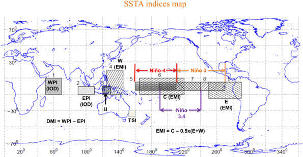
Figure 1. Map of the SSTA climate indices considered in this study.
Download figure:
Standard image High-resolution image2.3. Drift correction
We apply a drift correction to the indices calculated from the decadal experiments, as recommended for CMIP5 decadal predictions by Climate Variability and Predictability (CLIVAR) (WCRP 2011). This assumes that the drift in the monthly average prediction is just a function of the forecast lead time and is not affected by the model state or the external radiative forcing. For each model and index, bias for the 120 month period (obtained by comparing the model and the observed index values month wise), averaged across all ensembles and initializations, is assumed to represent the mean model drift. So the mean drift is different for each model and index and is subtracted from the index values obtained for individual decadal experiment of the model to give the drift corrected forecast. The uncorrected model forecasts are hereby referred to as raw forecasts.
2.4. Estimation of predictability horizon
The indices for each ensemble member and for the ensemble mean for each initialization time are compared with the concurrent observed indices in order to calculate the 120 month (decadal) time series of squared errors (for both the raw and drift-corrected forecast). An estimate of the lead time over which the indices are predictable is obtained by comparing the model errors with distributions of randomly generated errors. A Monte Carlo (MC) scheme is applied to generate twelve random error distributions, one for each calendar month. This is done since SST variance can vary seasonally and, as such, the distribution of errors changes by season. For each index and model, the squared errors for all the decades and ensemble members are averaged to produce the typical monthly evolution of model errors over a period of 120 months. Model errors for each lead time are compared against the appropriate random error distribution. The index is considered predictable at a certain lead time, if the error is smaller than 95% of the random error distribution, i.e., the predictable lead time is the month before the error is greater than 95% of the random error distribution (figure 2(b)). For instance, HadCM3 (i2) has 10 ensemble members, and we consider forty one decades (yearly intervals starting from 1960 to 2000, as mentioned earlier). The model squared errors are averaged across all decades (41) and ensembles (10), resulting in a single 120 month error time series for each of the indices. The MC scheme used here calculates the average of 410 (41 × 10) 120 month random error time series and repeats it 10 000 times to generate a probability distribution that is used as the climatology of the errors. The model squared errors and the error climatology are then compared (using a 5% significance level) to obtain the period of useful prediction, the predictability horizon. Errors associated with a persistence forecast are also calculated. Persistence is defined as the error that results if the index forecast is set to the initial value (i.e. set at the time of forecast initialization) throughout the forecast period. If the model forecast skill cannot exceed the persistence skill, then it has no merit.
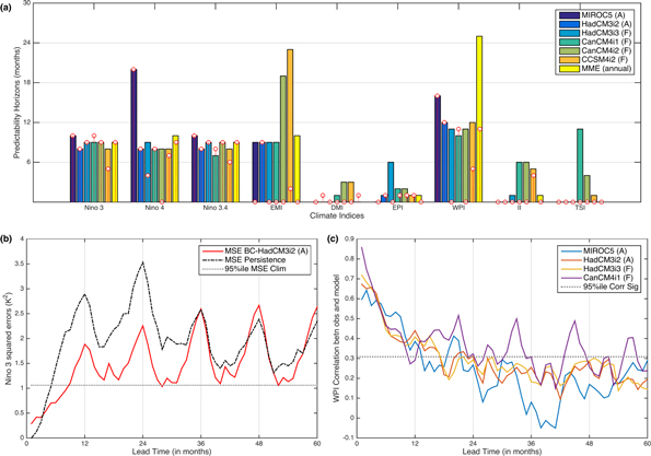
Figure 2. (a) Predictability horizon (months of useful predictability) based on Monte Carlo analysis for the nine SSTA climate indices, for drift corrected model forecasts. Results from raw model runs are shown in white circles (A—anomaly initialized; F—full-field initialized); MME (annual) stands for multi model ensemble mean calculated by considering only the models with annual initializations. (b) Multi-ensemble mean squared errors for Niño 3 based on drift corrected HadCM3i2 forecasts; persistence errors are shown in black; 95 percentile squared errors from the MC simulation shown in gray. (c) Sample time series of correlation between drift-corrected model WPI and observed WPI. Only models with annual initializations are shown. Gray line denotes the significance at 95% level with 39 degrees of freedom on the basis of one-side Student's t-test.
Download figure:
Standard image High-resolution image3. Analysis and results
3.1. Predictability horizon and drift correction
The predictability horizons (lead time in months) for the indices from the drift corrected and the raw model outputs are shown in figure 2(a). Drift correction leads to clear improvements for the full-field initialized models but improvements are not so evident in case of anomaly-initialized models, except for EMI. The indices in the tropical Pacific and the Western Indian Ocean have higher predictability horizons than other indices. For the ENSO related indices and WPI, MIROC5 shows the highest predictability horizon but shows no significant predictability, even at short lead times, for the DMI, EPI, II and TSI indices. The highest predictability horizons are noted for EMI, with an average of 13 months (range 9–23 months), and WPI, with an average of 12 months (range 10–16 months). EMI is discussed in further detail in section 4.2. The MME shows the highest predictability for WPI at 25 months. The Indian Ocean DMI has the poorest predictability horizon with a maximum of only three months.
We also estimated prediction lead times using a correlation analysis between the monthly observed and ensemble mean indices at each lag time (results for only WPI shown in figure 2(c)), which shows a similar trend as earlier with Pacific indices and the WPI showing higher skills than other indices while DMI shows the least, suggesting that our results are robust to the metric used. The predictability horizons shown in figure 2(a) are also broadly consistent with persistence forecast (where the forecast at all lead times is simply the initial value of that metric; see section 2.4). For a prediction to be useful, the associated error from the model should be smaller than both the 95% random error and the persistence forecast error. As an example, in figure 2(b), it can be seen that the HadCM3i2 Niño 3 prediction errors are lower than the persistence error for almost forty five months and lower than the MC climatology error for eight months supporting the predictability horizon obtained for this index.
Based on our analysis of the predictability horizons, the comparison of squared errors with persistence errors and correlations from this subset of models, no clear conclusion can be made regarding which type of initialization performs better. Indeed, previous studies (Magnusson et al 2012, Hazeleger et al 2013, Smith et al 2013) have not been able to identify a preferred initialization method for improving forecast quality at interannual to decadal timescales.
3.2. El Niño and La Niña prediction
The drift corrected Niño 3 and Niño 3.4 values obtained from the models are compared with those observed, for two decades containing large El Niño events of 1982/83 and 1997/98 and two decades containing the large La Niña events of 1973/74 and 1988/89. For the El Niño events, observed indices are compared with the indices obtained from model experiments initialized in 1981 and 1982 (for the 1982/83 El Niño) and 1996 and 1997 (for the 1997/98 El Niño), to see the effect of lead time on El Niño prediction. For the La Niña events, observed indices are compared with the indices obtained from model experiments initialized in 1972 and 1973 (for the 1973/74 La Niña) and 1987 and 1988 (for the 1988/89 La Niña), to see the effect of lead time on El Niño prediction. Only models with annual initializations are used for the analyses.
Results from the two models (HadCM3i2 and CanCM4i1) initialized one and two years before the 1997 and 1982 El Niño events are shown in figures 3(a), (b), (e) and (f). Results from the other two models are given in the supplementary material (figure S1). HadCM3i2 and CanCM4i1 show considerable skill in capturing both the El Niño events 9–12 months in advance, in figures 3(a) and (b). At the peak of the 1997 (1982) El Niño, 9 (7) out of 10 ensemble members of HadCM3i2 (A) and 10 (8) out of 10 ensemble members of CanCM4i1 (F), have positive Niño 3.4 anomalies. Comparing with a binomial distribution for 10 ensembles, these correspond to 99 (90) percentile for HadCM3i2 (A) and 100 (95) percentile for CanCM4i1 (F) during the peak of 1997(1982) El Niño. There is some indication that some models may provide useful information on the phase of ENSO at longer lags although the fraction of ensemble members agreeing might not be significant. For example, El Niño 1997 (1982) has 6 (7) out of 10 ensemble members of HadCM3i2 (A) and 4 (7) out of 10 ensemble members of CanCM4i1 (F) showing positive Niño 3.4 anomalies as shown in figures 3(e) and (f), which corresponds to 62 (83) percentile for HadCM3i2 (A) and 38 (83) percentiles.
Similar analyses are repeated for the La Niña events of 1988/89 (initializations 1987 and 1988) and 1973/74 (initializations 1972 and 1973; HadCM3i3 and CanCM4i1 in figures 3(c), (d), (g) and (h)); MIROC5 and HadCM3i2 in figure S2). When initialized 9–12 months before the events, as in figures 3(c) and (d), 9(10) out of 10 ensemble members of HadCM3i3 (F) and 10 (10) out of 10 ensemble members of CanCM4i1 (F), have negative Niño 3.4 anomalies, at the peak of the 1988 (1973) La Niña. These correspond to a significance level of more than 99 percentile for all the cases. For longer lead times, as shown in figures 3(g) and (h), 7 (4) out of 10 ensemble members of HadCM3i3(F) and 6 (6) out of 10 ensemble members of CanCM4i1(F) show negative Niño 3.4 anomalies. As in the case of El Niño prediction at such lead times, the fraction of ensemble members predicting the phase of the event correctly is still insignificant.
Despite most ensemble members predicting the phase of ENSO correctly, majority of them under-predict the magnitude (severity) of the El Niño and La Niña events, with the situation becoming worse at larger lead times. However, the two full-filled initialized models (CanCM4i1 and HadCM3i3) clearly outperform the anomaly initialized models (MIROC5 and HadCM3i2) in predicting these events. The MME shows poorer skills compared to the individual models in simulating these anomalies and thus are not shown. While the numbers of models/events are too small to reliably infer that full-field initialization produces consistently superior results to anomaly initialization for ENSO forecasts, our findings are in agreement with previous studies that have suggested that full-field initialized models are more skillful at seasonal timescales (Magnusson et al 2012, Meehl et al 2014).
4. Discussion
This study evaluates the predictive skill of multiple SSTA climate indices using the decadal prediction experiments of four CMIP5 models. All models showed the highest predictability for ENSO related metrics and the Western Indian Ocean SSTA. Similar results were also obtained from comparing the model squared errors for each of the indices with their respective persistence errors and from the correlation coefficients. Our results also show the initialized models to have varying degrees of skills in predicting El Niño and La Niña events at 1 or 2 year lead times. Some specific points from the analysis are discussed in greater detail below.
4.1. Drift correction
We have demonstrated that drift correction is critical prior to using decadal simulation outputs in the case of full-field initialization models. However, for the anomaly-initialized models there is little to no benefit gained from applying a drift correction (for the metrics investigated). Drift correction techniques are imperfect remedies for these model biases and are often considered as an additional source of uncertainty, as they might neglect significant statistical relationships between the variables (Ho et al 2012). More sophisticated techniques for drift correction may be able to extract greater predictability. Some examples of improved drift correction techniques could include post processing approaches like applying a time-dependent trend adjustment after the simple time-dependent bias adjustment (Kharin et al 2012) or forming a covariate model of drift correction using the sub-surface ocean heat content as a metric, but as mentioned earlier these need to be scrutinized properly before application.
4.2. SSTA predictability
Predictability on multi-year timescales for Pacific SSTs (and PDO) was reported by Chikamoto et al (2012) using the MIROC climate model. Mehta et al (2013) studied decadal predictability of SST from four Earth System Models and reported highest skill from MIROC5 and low and insignificant skills from HadCM3 and CCSM4 in the tropical Pacific. Chikamoto et al (2015) reported ENSO related prediction skill to decrease rapidly after lead times of one year from the MIROC5 model. Our results are consistent with these findings that MIROC5 has the highest predictability in the tropical Pacific. However, it shows limited skill in terms of simulating large climate anomalies like El Niños and La Niñas.
The significantly high predictability horizons noticed for EMI from CanCM4 (i2) and CCSM4 (i2) are attributed to issues from sampling variability resulting from the fact that these models have runs with start dates every 5 years and thus have only 9 set of decades. Also, given that EMI is a function of SSTA averaged across different parts of the Pacific Ocean, these sampling issues might get largely amplified. These sampling issues regarding initializations every year and initializations every five years requires thorough analysis and would be the subject of a different study.
4.3. Implications for regional rainfall
Chiew et al (1998) and many others suggest significant link between spring and summer rainfall over Northeast Australia with ENSO and winter rainfall over Northwest Australia with indices in the Indian Ocean. To investigate the implication of index predictability on regional rainfall prediction, we calculate correlations between area-averaged rainfall and the corresponding drift-corrected SSTA index forecast at lead times of 10–12 (6–8) and 22–24 (18–20) months for the spring–summer (winter) rainfall values. The concurrent correlation between the observed index and rainfall is also shown for comparison. Rainfall data is from the Australian Bureau of Meteorology monthly gridded rainfall dataset (Jones et al 2009).
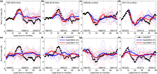
Figure 3. (a) Niño 3.4 values simulated by HadCM3i2 (blue) and CanCM4i1 (red) initialized in 1997 along with the HadISST Niño 3.4 values (black) during 1996–2000. Individual model ensembles (10 each) are lightly colored in the background with the ensemble means thickened. (b) Niño 3.4 values simulated by HadCM3i2 (blue) and CanCM4i1 (red) initialized in 1982 along with the HadISST Niño 3.4 values (black) during the decade 1981–1985. Individual model ensembles (10 each) are lightly colored in the background with the ensemble means thickened. (c) Niño 3.4 values simulated by HadCM3i3 (blue) and CanCM4i1 (red) initialized in 1988 along with the HadISST Niño 3.4 values (black) during 1987–1991. Individual model ensembles (10 each) are lightly colored in the background with the ensemble means thickened. (d) Niño 3.4 values simulated by HadCM3i3 (blue) and CanCM4i1 (red) initialized in 1973 along with the HadISST Niño 3.4 values (black) during 1972–1976. Individual model ensembles (10 each) are lightly colored in the background with the ensemble means thickened. (e) Same as (a) except model simulations initialized in 1996. (f) Same as (b) except model simulations initialized in 1981. (g) Same as (c) except model simulations initialized in 1987. (h) Same as (d) except model simulations initialized in 1972.
Download figure:
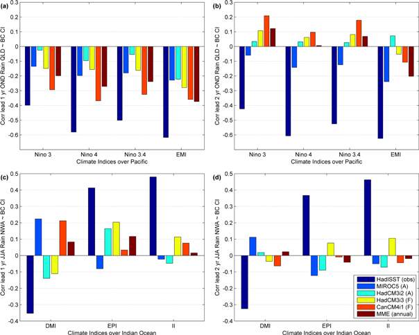
Standard image High-resolution imageFigure 4 shows the correlations between area averaged Oct–Nov–Dec (OND) rainfall over Queensland with the concurrent observed and drift-corrected Pacific SSTA indices, and Jun–Jul–Aug (JJA) rainfall over North Western Australia with the concurrent observed and drift-corrected Indian Ocean SSTA indices within lead times extending to a maximum of one and two years. Only models with annual initializations are considered so that there are enough samples to provide reliable correlation estimates. There are strong negative correlations between the observed Pacific indices and area-averaged OND rainfall over Queensland highlighting the relationship between ENSO and Northeast Australian spring–summer rainfall. All the models are able to reproduce this negative relationship, although the correlations become non-significant after a lead time of 10 months, which is consistent with the predictability horizons. For the Indian Ocean, there are strong observed positive correlations between area-averaged JJA rainfall over North Western Australia with EPI and II and negative correlations with DMI. The models do not consistently reproduce these relationships, suggesting that the Indian Ocean provides little useful predictable skill even at lead times less than a year.
Figure 4. (a) Correlation of area-averaged Oct–Nov–Dec rainfall over Queensland with climate indices in the Pacific from the observed and lead 10–12 months drift-corrected model values; MME (annual) stands for multi model ensemble mean calculated by considering only the models with annual initializations. (b) Same as (a) but for model values at lead 22–24 months. (c) Correlation of area-averaged June–July–August rainfall over North Western Australia with climate indices in the Indian Ocean from the observed and lead 6–8 months drift-corrected model values. (d) Same as (c) but for model values at lead 18–20 months.
Download figure:
Standard image High-resolution image
Numerous studies have reported significant link between SSTA over the Western Indian Ocean and East African rainfall (Ummenhofer et al 2009b, Black 2005). Our study shows all models and the MME having high predictability horizons for WPI. This result along with the analysis for figure 4 show the potentiality of rainfall prediction using the drift corrected model forecasts of these SSTA indices at seasonal to annual timescales. However, this also presents the need of using improved methods of rainfall prediction for a practical application of the SSTA indices from the CMIP5 decadal experiments.
5. Conclusions
Forecasting rainfall at seasonal and longer timescales is of great societal importance. However, climate models have large biases in their representation of rainfall in part related to problems in the simulation of realistic teleconnections from climate drivers such as ENSO and regional rainfall. Thus instead of looking at simulated rainfall, we have examined predictions of SSTA indices which have significant relationships with regional rainfall. We find that while these models are unable to predict interannual variations beyond about a year, they have considerable skill at shorter timescales, similar to bespoke seasonal forecasting systems. There is a clear divide in the predictability of Pacific indices and WPI compared to indices in the Indian Ocean, which show little predictability. This is also evident in the strength of the relationships between rainfall in two regions of Australia with the observed and modeled Indian and Pacific Ocean indices. Based on only two events and two models for each initialization type, full-field initialized models seem to outperform the anomaly initialized ones in simulating ENSO related anomalies at annual timescales. The recommended drift correction has negligible effect on anomaly initialized models but is critical for full-field initialized models and improved drift correction techniques may provide further improvements. Future works will, therefore, focus on investigating such advanced drift correction techniques and estimating the skill of rainfall prediction at longer than seasonal timescales from the CMIP5 decadal experiments.
Acknowledgments
The World Climate Research Program's Working Group on Coupled Modeling is responsible for CMIP. We thank the climate modeling groups for producing and making available their model outputs used in our study (see table S1, accessible online through http://pcmdi9.llnl.gov/esgf-web-fe/). For CMIP, the US Department of Energy's Program for Climate Model Diagnosis and Intercomparison provides coordinating support and led development of software infrastructure in partnership with the Global Organization for Earth System Science Portals. We acknowledge the Australian Research Council (ARC) for funding this research. We also acknowledge the support and encouragement from the Australian Bureau of Meteorology and the New South Wales State Water Corporation.