

Abstract
Tropical forests provide global climate regulation ecosystem services and their clearing is a significant source of anthropogenic greenhouse gas (GHG) emissions and resultant radiative forcing of climate change. However, consensus on pan-tropical forest carbon dynamics is lacking. We present a new estimate that employs recommended good practices to quantify gross tropical forest aboveground carbon (AGC) loss from 2000 to 2012 through the integration of Landsat-derived tree canopy cover, height, intactness and forest cover loss and GLAS-lidar derived forest biomass. An unbiased estimate of forest loss area is produced using a stratified random sample with strata derived from a wall-to-wall 30 m forest cover loss map. Our sample-based results separate the gross loss of forest AGC into losses from natural forests (0.59 PgC yr−1) and losses from managed forests (0.43 PgC yr−1) including plantations, agroforestry systems and subsistence agriculture. Latin America accounts for 43% of gross AGC loss and 54% of natural forest AGC loss, with Brazil experiencing the highest AGC loss for both categories at national scales. We estimate gross tropical forest AGC loss and natural forest loss to account for 11% and 6% of global year 2012 CO2 emissions, respectively. Given recent trends, natural forests will likely constitute an increasingly smaller proportion of tropical forest GHG emissions and of global emissions as fossil fuel consumption increases, with implications for the valuation of co-benefits in tropical forest conservation.
Export citation and abstract BibTeX RIS

Content from this work may be used under the terms of the Creative Commons Attribution 3.0 licence. Any further distribution of this work must maintain attribution to the author(s) and the title of the work, journal citation and DOI.
1. Introduction
Deforestation and degradation of tropical forests constitute the second largest source of anthropogenic emissions of carbon dioxide after fossil fuel combustion (van der Werf et al 2009). Policy initiatives have been proposed to reduce the rate of tropical forest loss, which would have the co-benefit of preserving other unique tropical ecosystem services such as biodiversity richness (Jantz et al 2014). The REDD+ mechanism under the United Nations Framework Convention on Climate change (UNFCCC) seeks to compensate developing countries for avoided emissions that would have otherwise occurred under business as usual scenarios. To do so, methodologically consistent baseline estimates of forest carbon stocks and forest loss area within different forest types are required as a part of national forest monitoring systems, which is underlined by the recent decision of the UNFCCC Conference of the Parties 19 (COP 19) on 'Modalities for national forest monitoring systems' (UNFCCC 2014). Existing estimates of gross carbon loss derived from carbon stock and forest area loss data vary greatly (from 0.81 to 2.9 PgC annually (Pan et al 2011, Harris et al 2012, Achard et al 2014)) with the greatest variance found between studies that employ remotely sensed-derived data versus those that use forest inventory and other tabular reference data. Aggregate emissions from deforestation based largely on satellite-derived products are similar (∼0.81 PgC) despite regional differences (Houghton 2013) in pan-tropical carbon density reference data, forest cover change estimates, and the carbon pools included (Saatchi et al 2011, Houghton 2013, IPCC 2013, Mitchard et al 2013, Ometto et al 2014).
For REDD+ purposes, countries are required to report GHG emissions and removals by different types of human activities (e.g. forestry, agriculture and other land use); the extent of these activities is called 'activity data' and is reported in units of area. Activity data are combined with emissions factors to generate emissions estimates. If a map is to be used to estimate activity data, its accuracy must be quantified. Good practice guidance from the Intergovernmental Panel on Climate Change (IPCC) requires emissions estimates to neither over- nor under-estimate as far as can be judged, and to have uncertainties reduced as far as practicable (IPCC 2003). Methodological guidance from the Global Forest Observations Initiative (GFOI) suggests that 'to satisfy these criteria, compensation should be made for classification errors when estimating activity areas from maps and uncertainties should be estimated using robust and statistically rigorous methods. The primary means of estimating accuracies, compensating for classification errors, and estimating uncertainty is via comparisons of map classifications and reference observations for an accuracy assessment sample' (GFOI 2014). To this end, we demonstrate a generic and cost-effective approach for estimating forest cover loss activity data that follows good practice guidance (IPCC 2006, GFOI 2014, Olofsson et al 2014). We achieve this by using an existing forest cover loss map (Hansen et al 2013) to allocate samples in the quantification of activity data pan-tropically. Per good practice guidance, the sample supersedes the map in the estimation of forest area loss. The map, however, is critical in the efficient allocation of the sample population and results of the sample-based estimate can be used to validate the map-based estimate. Probability-based sample is required to meet the standard of statistical rigor in estimating forest cover loss area and associated uncertainty; the demonstrated approach represents the most rigorous assessment of pan-tropical forest loss activity data to date.
Gross carbon loss due to removal of aboveground forest biomass in 2000–2012 is quantified in a 'stratify and multiply' (stock-difference) approach (Goetz et al 2009) in which area of forest loss is first estimated and then the aboveground carbon (AGC) density associated with loss areas quantified. In this study, the strata of the 'stratify and multiply' approach were forest carbon stock strata based on canopy structure as defined by percent cover (Hansen et al 2013) and height, and intactness (Potapov et al 2008). Within each forest carbon stock stratum, forest cover loss and no loss sub-strata were defined using a pan-tropical subset of mapped global forest cover loss from 2000 to 2012 (Hansen et al 2013). The area of forest loss was estimated from a probability sample for which forest loss was determined using visual interpretation of Landsat time series and high resolution imagery from Google EarthTM at each sample location. The AGC density estimates were obtained based on field-calibrated LIDAR estimates of aboveground biomass (Baccini et al 2012) and associated with the carbon stock strata. This approach was prototyped earlier at the national scale for the Democratic Republic of the Congo (Tyukavina et al 2013), and can be implemented at various geographic scales given the appropriate data on forest type, forest loss and carbon density, which makes it potentially useful for national forest monitoring systems. The data used in the analysis are freely available, obviating the need for commercial data sets that are often too costly and consequently impractical to incorporate into operational national-scale forest monitoring programs.
This study defines forest as any vegetation taller than 5 m with canopy cover ≥25% (both natural forests and plantations); this corresponds to the forest definition agreed under the UNFCCC (UNFCCC 2006) except for the minimum area and potential for growth criteria: 'Forest' is a minimum area of land of 0.05–1.0 hectare with tree crown cover (or equivalent stocking level) of more than 10–30 per cent with trees with the potential to reach a minimum height of 2–5 m at maturity in situ.' Forest cover loss is defined as any stand-replacement disturbance (Hansen et al 2013), both semi-permanent conversion of forest cover into other land cover and land use types ('deforestation' as defined by FAO (FAO 2012) and under the UNFCCC (UNFCCC 2006)) and temporary forest disturbances followed by tree regeneration.
An advantage of sample-based estimation is the possibility of attributing additional contextual information to each sample, for example land use. Considerable forest cover loss in the tropics is due to established land use practices, included forestry and shifting cultivation. Given the importance of natural forests to carbon stocks, biodiversity, and other ecosystem services, we further disaggregate sample-based gross forest cover and AGC loss into occurring in natural (primary and mature secondary forests, and natural woodlands) and managed (tree plantations, agroforestry systems, areas of subsistence agriculture with rapid tree cover rotation) forests (see section 2 and figure 4). Natural forest cover loss represents forests cleared for the first time in recent history and is the primary target of initiatives such as REDD+. This category of AGC loss can be applied to cases where natural forests are replaced by non-forestry land uses (deforestation), such as the conversion of Amazonian rainforests to pastures, where natural forests are replaced by forestry land uses, such as the conversion of Sumatran rainforests to forest plantations, and where natural forests are cleared and incorporated into shifting cultivation landscapes to be replaced by secondary regrowth, such as in the Congo Basin. Natural forests, as defined in this study, represent the comparatively intact remaining tropical forest ecosystems. It is posited here that natural forests are a limited, non-renewable resource and that quantifying their contribution to the overall emissions dynamic is valuable in informing policy initiatives such as REDD+.
We estimate gross AGC loss due to stand-replacement disturbance mapped at a 30 m resolution and add a modeled belowground carbon loss (BGC) estimate in order to compare results with other contemporary remote-sensing based studies. Forest disturbances often associated with forest degradation include burning, selective logging, forest fuelwood removal, and charcoal production (Cochrane and Schulze 1999). Our study quantifies these dynamics where observable, including forest loss due to fire and the building of roads and other infrastructure associated with selective logging, but does not account for the finer scale disturbances that cannot be directly mapped using Landsat data, largely selective removals due to logging. Pearson et al (2014) recently found that in countries with high rates of deforestation such as Indonesia and Brazil, carbon emissions from selective logging account for ∼12% of emissions from deforestation, including losses due to infrastructure.
2. Data and methods
2.1. Study region
Our study region includes biomes within tropical, subtropical and portions of the temperate climate domains in Latin America between 30°N and 60°S, in Sub-Saharan Africa between 30°N and 40°S and in South and Southeast Asia between 40°N and 20°S. Our forest cover stratification was produced within this area. For the final forest cover loss area and AGC loss estimation, we limited our study area to the following countries and country groups (figure 1):
- (1)Africa: Democratic Republic of the Congo, humid tropical Africa, the rest of Sub-Saharan Africa.
- (2)Latin America: Brazil, Pan-Amazon, the rest of Latin America.
- (3)South and Southeast Asia: Indonesia, mainland South and Southeast Asia, insular Southeast Asia.
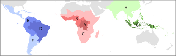
Figure 1. Boundaries of reporting units. (A) Democratic Republic of the Congo; (B) humid tropical Africa; (C) the rest of Sub-Saharan Africa; (D) Brazil; (E) Pan-Amazon; (F) the rest of Latin America; (G) Indonesia; (H) mainland South and Southeast Asia (includes southern China up to 40°N); (I) insular Southeast Asia.
Download figure:
Standard image High-resolution image2.2. Approach to estimating gross AGC loss
The 'stratify and multiply' approach (Goetz et al 2009) to estimating gross AGC loss was implemented using the basic IPCC (2006) equation:

where AD denotes activity data, the extent of human activity, and EF denotes emissions factors, the emissions or removals per unit activity.
Modifying this basic equation for the estimation of AGC loss we obtain:
where i denotes a forest cover type (forest stratum), ADi is forest cover loss within forest type i, EFi is mean AGC density for forest type i, and the summation is over all forest types.
We used the following data to estimate 2000–2012 AGC loss using this approach:
- (1)Forest cover type stratification for year 2000 (prior to disturbance).
- (2)Forest cover loss map (AD) and validation sample data.
- (3)Mean carbon density estimate for each forest stratum (EF).
We estimated uncertainties from both AD and EF and incorporated them into the final AGC loss estimates using the recommended Approach 1 (Propagation of Error) from the IPCC Guidelines (IPCC 2006).
2.3. Pan-tropical forest cover stratification (year 2000)
The purpose for stratifying forest cover was to delineate regions (strata) associated with different carbon stock (EF) reference values. However, consistently characterized pan-tropical forest type maps are not available at the 30 m spatial resolution corresponding to the Hansen et al (2013) forest loss data. Characterizing forest cover based on complex multi-parameter definitions (e.g. 'primary forests', 'secondary forests', 'woodlands') as we have performed at a national scale (Potapov et al 2012, Tyukavina et al 2013) is not easily achieved at a biome scale. Instead, we defined tropical forest strata using remotely sensed-derived structural characteristics of tree canopy (year 2000 percent tree canopy cover (Hansen et al 2013)), tree height (current study) and forest intactness (Potapov et al 2008).
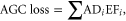
Stratification thresholds were developed to minimize within-strata AGC variance using a statistical regression tree approach with point-based GLAS carbon estimates (Baccini et al 2012) for the period 2003–2008 as the dependent variable. When building a tree, the highest priority was assigned to tree canopy cover, with height and intactness as auxiliary variables having lower weights in the model. Figure 2 shows the resulting regression tree. Only areas where tree canopy cover was ≥25% were considered forest cover and included in the final stratification (figure 3). Original 30 m forest strata are available for download from http://glad.geog.umd.edu/pantropical.
Figure 2. Forest cover stratification thresholds. Terminal node values are mean strata AGC density values (MgC ha−1).
Download figure:
Standard image High-resolution image
Figure 3. Forest cover stratification. (a) Africa; (b) South and Southeast Asia; (c) Latin America; numbers in the legend refer to forest strata: 1—low cover; 2—medium cover short; 3—medium cover tall; 4—dense cover short; 5—dense cover short intact; 6—dense cover tall; 7—dense cover tall intact.
Download figure:
Standard image High-resolution image2.4. Height model
Our tree height map was generated using a regression tree model which related GLAS-derived tree height estimates (Baccini et al 2012) to Landsat time-series metrics. Landsat 7 Enhanced Thematic Mapper Plus (ETM+) growing season images were processed to create a per-pixel set of cloud-free land observations which in turn were used to assemble the time-series metrics (Potapov et al 2012). Circa year 2000 tree height was derived by taking the maximum of five annual height models (2000–2004). A random subset of 90% of the available GLAS data was used to train models with the remaining 10% of the data set aside for cross-validation. For the study region the resulting five year maximum height model has root mean square error (RMSE) of 8.1 m and mean absolute error (MAE) of 5.9 m; within forests (crown cover >25%) RMSE = 6.5 m and MAE = 4.7 m.
2.5. Forest cover loss data
Per good practice guidance (Olofsson et al 2014), a sample-based approach (Cochran 1977) is required to estimate area of gross forest cover loss (Stehman 2013). Commission and omission errors inherent in the Hansen et al (2013) map likely introduce bias to the map-based forest loss area estimates. Consequently, we base the area estimates on the reference condition of each pixel selected in a sample; the reference sample condition is considered the most accurate available assessment of forest loss (the protocol for determining the reference sample condition is described later in this subsection). The global 2000–2012 forest cover loss map (Hansen et al 2013) was used to target reference samples in estimating area of forest cover loss. The use of a stratified estimator (Cochran 1977) substantially reduces standard errors relative to what would have resulted without stratification (Hansen et al 2008, Broich et al 2009). The global forest cover loss data are defined as all stand-replacement disturbances of vegetation taller than 5 m observable at a 30 m resolution. For the current analysis we considered only forest cover loss within the target forest strata (figure 3) with crown cover ≥25%. The 30 m forest cover loss data were used to create two sub-strata within each of the forest carbon stock strata of figure 3: one-pixel buffered forest cover loss (i.e., all map forest loss pixels and any pixels adjacent to a mapped loss pixel) and no loss (table 1). We created a one-pixel buffer around mapped loss to target forest loss omission error pixels that commonly occur at the boundary of map loss pixels (Tyukavina et al 2013).
Table 1. Sample size allocation per stratum for the stratified random sample. Forest strata codes are from figure 3: 1—low cover; 2—medium cover short; 3—medium cover tall; 4—dense cover short; 5—dense cover short intact; 6—dense cover tall; 7—dense cover tall intact.
| Sub-strata | ||
| Forest type strata | No loss | 1-pixel buffered loss (2000–2012) |
| Africa | ||
| 1, 2 | 130 | 60 |
| 3 | 130 | 60 |
| 4 | 130 | 60 |
| 5, 7 | 90 | 50 |
| 6 | 130 | 60 |
| Total sample size | 900 | |
| Latin America | ||
| 1, 2, 3 | 245 | 105 |
| 4, 6 | 350 | 150 |
| 5, 7 | 245 | 105 |
| Total sample size | 1200 | |
| South and Southeast Asia | ||
| 1, 2 | 65 | 25 |
| 3 | 135 | 45 |
| 4 | 185 | 90 |
| 5, 7 | 105 | 50 |
| 6 | 135 | 65 |
| Total sample size | 900 | |
In our previous validation effort (Hansen et al 2013), a sample of 300 120 m × 120 m sample units was allocated to the tropical biome to assess the accuracy of the forest cover map. However, this sample was deemed inadequate for the current analysis because several smaller forest carbon stock strata would have insufficient sample sizes and consequently large standard errors for the forest cover loss area estimates.
The current sample consisted of 3000 30 m pixels selected from the three tropical forest regions (table 1), with the sample size allocated to each region roughly proportional to their respective areas of forest cover loss, with 1200 sample pixels allocated to Latin America, and 900 sample pixels each to Africa and Asia. Separate per-continent sample allocations reduced continent-level standard errors for estimates of area of forest cover loss and overall accuracy (Stehman 2009). Forest carbon stock strata covering relatively small areas were combined into larger strata (table 1) for selecting the sample. Estimates of forest cover loss area were still obtained for every forest type displayed in figure 3. Forest cover loss area estimates were also made for select countries and country groups (see figure 1). These estimates were based on 2936 of the sample pixels; 64 sample pixels (15 in America and 49 in Asia) were excluded as they were outside of the countries of interest. Table 2 shows the sample size for each country and country group.
Table 2. Sample size allocation per countries and country groups (figure 1) for the final reporting.
| Reporting units | N of samples |
|---|---|
| Democratic Republic of the Congo | 328 |
| Humid tropical Africa | 298 |
| The rest of Sub-Saharan Africa | 274 |
| Brazil | 603 |
| Pan-Amazon | 337 |
| The rest of Latin America | 245 |
| Indonesia | 248 |
| Mainland South and Southeast Asia | 430 |
| Insular Southeast Asia | 173 |
The reference 2000–2012 forest cover loss condition (i.e., loss or no loss) was assigned to each sample pixel based on the visual interpretation of Landsat multitemporal composites for years circa 2000, 2003, 2006, 2009, 2012 and 2000–2012 maximal reflectance value composite, and high resolution imagery available through Google EarthTM. Of the 3000 sampled pixels, 1042 had at least one high resolution image available for the study period, 438 sample pixels had at least two images, and 219 sample pixels had three or more images. The validation process is illustrated schematically in figure 4. The full error matrix is presented in table S1.
The sample data were used to estimate area of forest loss by the seven forest cover types per continent (table S2), country and country group (table 3), and to calculate standard errors and the corresponding 95% confidence intervals of the estimates (Cochran 1977). The sample data were also used to estimate the proportion of loss occurring within natural forests (table 3, table S2). To obtain the latter estimates, each sample pixel that was identified as 2000−2012 loss was characterized as having occurred within 'natural' or 'managed' forest based on interpretation of Landsat time-series, high resolution data, and ancillary land cover information (figure 4, table S1). The 'natural' forest category included all primary and mature secondary forests and natural woodlands without evidence of prior disturbances. The 'managed' forest category included forest plantations, agroforestry systems and areas of subsistence farming due to shifting cultivation practices. In Landsat imagery, dense natural tropical forests with large crowns have coarser texture, while the texture of dense plantations composed of more uniform stands is comparatively smoother (figure 4). In the dry tropics, plantations often have denser canopy cover than natural vegetation and look brighter and more uniform in satellite imagery.
Table 3. 2000−2012 forest cover loss and aboveground carbon (AGC) loss estimates. The 'Sample estimate' value is computed using an unbiased estimator of forest cover loss area applied to data obtained from a probability sampling design (see section 2). Uncertainty is expressed as a 95% confidence interval (CI). For the boundaries of the regions see figure 1.
| Gross forest cover loss | Natural forest cover loss | Gross AGC loss | Natural forest AGC loss | ||||||
|---|---|---|---|---|---|---|---|---|---|
| Area (Mha) | |||||||||
| Map (Hansen et al 2013) | Sample estimate | Difference between sample and map estimates (%) | Area (Mha) | % of sample gross forest loss estimate | Annual (TgC yr−1) | Annual (TgC yr−1) | % of gross AGC loss | ||
| A | DRC | 5.9 | 9.7 ± 3.1 | ↑65 | 4.3 ± 1.9 | 45 | 86 ± 19 | 46 ± 12 | 53 |
| B | Humid Tropical Africa | 5.1 | 9.8 ± 6.2 | ↑92 | 1.2 ± 0.8 | 12 | 56 ± 29 | 12 ± 2 | 22 |
| C | The rest of Sub-Saharan Africa | 9.7 | 17.4 ± 6.2 | ↑79 | 9.0 ± 3.4 | 52 | 92 ± 27 | 47 ± 15 | 50 |
| Africa total | 20.7 | 36.9 ± 9.2 | ↑78 | 14.5 ± 4.9 | 39 | 234 ± 44 | 104 ± 21 | 45 | |
| D | Brazil | 34.4 | 37.6 ± 3.0 | ↑9 | 25.1 ± 3.8 | 67 | 266 ± 18 | 202 ± 12 | 76 |
| E | Pan-Amazon | 9.0 | 10.8 ± 1.8 | ↑21 | 7.5 ± 2.1 | 70 | 76 ± 14 | 58 ± 2 | 76 |
| F | The rest of Latin America | 14.9 | 18.8 ± 4.1 | ↑27 | 11.6 ± 3.6 | 62 | 99 ± 25 | 55 ± 15 | 56 |
| Latin America total | 58.3 | 67.3 ± 6.1 | ↑15 | 44.0 ± 5.7 | 65 | 442 ± 33 | 316 ± 21 | 72 | |
| H | Indonesia | 15.7 | 14.4 ± 2.0 | ↓9 | 7.5 ± 2.2 | 52 | 151 ± 14 | 88 ± 21 | 59 |
| I | Mainland South and Southeast Asia | 12.3 | 16.3 ± 2.8 | ↑32 | 10.3 ± 2.2 | 63 | 136 ± 23 | 90 ± 17 | 66 |
| G | Insular Southeast Asia | 6.1 | 5.5 ± 1.3 | ↓9 | 2.7 ± 1.5 | 49 | 58 ± 12 | 32 ± 15 | 54 |
| South and Southeast Asia total | 34.2 | 36.4 ± 3.8 | ↑6 | 18.9 ± 4.5 | 52 | 346 ± 32 | 167 ± 39 | 48 | |
| Pan-tropical total | 113.1 | 140.5 ± 11.6 | ↑24 | 77.5 ± 8.8 | 55 | 1022 ± 64 | 588 ± 49 | 58 | |

Figure 4. Validation samples (small red squares): (a)–(g)—natural forest loss in Mato Grosso, Brazil; (h)–(n)—plantation clearing and regrowth in Parana, Brazil; (a)–(f) and (h)–(k) are Landsat multitemporal composites for years circa 2000, 2003, 2006, 2009, 2012 and 2000–2012 maximal composite; (g),(n)—high resolution imagery from Google EarthTM.
Download figure:
Standard image High-resolution image2.6. Carbon density data
Baccini et al (2012) employed field data and co-located GLAS lidar data to convert GLAS waveform metrics into biomass estimates. The field-calibrated statistical relationships were then applied to approximately 9 million tropical GLAS shots between 23°N and 23°S in a semi-regular grid of ICESat tracks (figure 6). We employed the field-calibrated GLAS-derived biomass data to calculate continent-specific mean strata AGC densities (figure 5, figures 7(a)–(c) and table S2). In effect, we treated the GLAS biomass data in this study as a substitute for field inventory data. Regression model errors from Baccini et al (of 22.6 MgC ha−1; 5.5%) were not incorporated into calculations; the uncertainty of mean strata AGC estimates was characterized by their standard errors calculated from GLAS samples. The biomass data used in this study are not from the map product of Baccini et al (2012), but from the population of GLAS shots converted to biomass used in generating the carbon stock map of Baccini et al (figure 6). Mean AGC densities for each stratum were averaged from a very large number of GLAS observations (hundreds of thousands observations each), which yielded small standard errors (figure 5) and offset the impact of the outliers in the GLAS-derived biomass data (see the scale bar of figure 6).
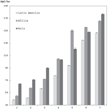
Figure 5. Mean AGC densities (±95% CI) for forest strata 1–7 within the three study regions, derived from GLAS-modeled biomass samples (Baccini et al 2012).
Download figure:
Standard image High-resolution image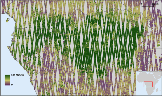
Figure 6. GLAS samples (2003−2009) attributed with aboveground carbon (AGC) densities. Each circle on the map corresponds to a ∼65 m diameter circular GLAS lidar footprint with the modeled AGC density (MgC ha−1) value (Baccini et al 2012).
Download figure:
Standard image High-resolution imageOur main result is AGC loss, for which we employ a source of AGC stock in the form of biomass-calibrated lidar data; these data serve as a surrogate for forest inventory measurements with mean and variance calculated per our mapped carbon stock strata. Though we have no analogous observational data for BGC, we further estimated per-stratum BGC densities and BGC loss in order to make our results comparable to those of Harris et al and Achard et al Stratum-specific BGC densities were estimated from AGC densities using equation 1 from Mokany et al (2006), and uncertainty of BGC using equation S7 from Saatchi et al (2011).
3. Results
We estimate gross AGC loss in the entire pan-tropical region to be 1022 ± 64 TgC yr−1 (table 3, figure 7(d)–(f)). AGC loss within natural forests accounted for 58% of the estimated total pan-tropical AGC loss and differed among the study regions (table 3, figure 8) with the highest losses in the Amazon basin and the lowest in Central Africa. Latin America experienced the highest AGC loss of the three regions of study, accounting for 43% of gross and 54% of natural forest pan-tropical AGC loss. Brazil alone accounted for 26% of pan-tropical gross forest AGC loss and 34% of natural forest AGC loss. Africa experienced the least AGC loss among continents, totaling one-half of Latin America's gross and one-third of its natural AGC loss. AGC loss within intact forests (strata 5 and 7, see table S2) accounted for 11% of the pan-tropical total, 70% of which occurred in Latin America.

Figure 7. Forest strata average aboveground carbon (AGC) density and loss: (a)–(c), year 2000 aboveground carbon (AGC) density; (d)–(f), estimated 2000–2012 AGC loss. Data are aggregated to 5 km for display purposes.
Download figure:
Standard image High-resolution image
Figure 8. Forest loss in natural and managed forests. Sample locations classified as reference loss within natural and managed forests for each of the seven forest type strata (see figure 3): 1—low cover; 2—medium cover short; 3—medium cover tall; 4—dense cover short; 5—dense cover short intact; 6—dense cover tall; 7—dense cover tall intact.
Download figure:
Standard image High-resolution image
AGC loss is dominant in dense forests (strata 4–7, see table S2), which accounted for 82% of gross forest AGC loss and 86% of natural forest AGC loss in Latin America, and 86% of gross and 95% of natural forest AGC loss in South and Southeast Asia. Dense forests in Africa accounted for 41% of gross and 62% of African natural forest AGC loss, meaning AGC loss in savanna woodlands is comparable to that of humid tropical forests in Africa. Proportional AGC loss per unit area of forest is higher in natural forests for all humid tropical-dominated regions. Sub-regions with significant dry tropical forest and woodland cover (regions C and F; table 3) have proportionately less AGC loss within natural forests compared to managed systems, likely reflecting the presence of plantations with higher carbon stock than native tree cover. Our AGC + BGC loss results are displayed in table 4 and show a 27% increase over AGC loss alone.
Table 4. Comparison of gross carbon loss estimates. AGC stands for aboveground carbon; BGC—belowground carbon. Range of uncertainty represents the 95% confidence interval for the current study; 90% prediction interval derived from Monte Carlo simulations and including all critical sources of uncertainty for Harris et al (2012), and uncertainty range derived from a sensitivity analysis related to the bias in carbon density maps for Achard et al (2014).
| Annual gross loss (TgC yr−1) | |||||||||
|---|---|---|---|---|---|---|---|---|---|
| AGC | AGC + BGC | AGC + BGC | |||||||
| Current study | Current study | Harris et al 2012 | Achard et al 2014 | ||||||
| Period (2000s) | Estimate | Range | Estimate | Range | Median | Range | Average | Range | |
| Africa | 00–05 | 116 | 54–218 | 148 | 44–221 | ||||
| 05–10 | 234 | 190–278 | 300 | 252–348 | — | — | |||
| 10–12 | — | — | — | — | |||||
| Latin America | 00–05 | 440 | 309–674 | 465 | 323–650 | ||||
| 05–10 | 442 | 409–475 | 564 | 518–610 | — | — | |||
| 10–12 | — | — | — | — | |||||
| South and Southeast Asia | 00–05 | 257 | 208–345 | 267 | 236–367 | ||||
| 05–10 | 346 | 314–378 | 439 | 397–481 | — | — | |||
| 10–12 | — | — | — | — | |||||
| Pan-tropical total | 00–05 | 813 | 570–1220 | 880 | 602–1237 | ||||
| 05–10 | 1022 | 958–1086 | 1303 | 1225–1381 | — | — | |||
| 10–12 | — | — | — | — | |||||
Total forest cover loss estimated from the reference classification of loss or no loss for the validation sample was higher compared to the estimated loss area obtained from the Hansen et al (2013) forest loss map for each of the three study regions (table 3 and table S2). The largest increase was observed in Africa (78%). Tyukavina et al (2013) reported a similar finding for the Democratic Republic of Congo, largely due to the scale of disturbance in smallholder landscapes and a resulting omission of forest loss. Landsat's 30 m spatial resolution was more appropriate for accurately quantifying the industrial-scale clearings of South America and Southeast Asia. The analysis of spatial distribution of forest loss confirms this interpretation: the ratio of the area of one-pixel boundaries around forest loss to the area of loss is 2.2 in Africa, 1.3 in South and Southeast Asia and 1.0 in Latin America. The ratio differs even more when comparing individual countries: 2.2 in the DRC, 0.88 in Indonesia and 0.79 in Brazil. For small-scale change dominated regions such as Africa, Landsat resolution assessments of forest change may lead to significant underestimation of forest carbon loss (Tyukavina et al 2013). Forest cover loss in the initial map was underestimated predominantly in forests with low canopy cover (strata 1 and 2, table S2), where the forest change signal is more ambiguous from the remote sensing perspective. Dry tropical forests are less well-studied than humid tropical forests and improved forest cover change mapping approaches are required to monitor the extent and change of open canopied woodlands and savannas.
4. Discussion and conclusions
The most directly comparable antecedent studies (Harris et al 2012, Achard et al 2014) estimated total above- and BGC-loss for the tropical region (table 4). These two studies and the presented one each vary in geographic and temporal extent, as well as observational inputs and methods for both carbon loss and associated uncertainty (table S3). Our carbon loss totals are higher than that of Harris et al and Achard et al, with our pan-tropical and regional Africa and Southeast Asia gross carbon loss estimates outside of the range of the previous studies (table 4). Of the various differences in the three tropical forest carbon loss studies, possibly the most significant is the study period. Results from Hansen et al indicated an increasing rate of forest cover loss within the 2000–2012 period. The study of Harris et al covered 2000–2005 and Achard et al covered 2000–2010. The inclusion of more recent years experiencing more forest cover loss is a likely source of difference in the respective carbon loss estimates. Additionally, our carbon stock data are not coarse resolution maps of biomass as in the previous studies. For example, Baccini et al (2012), which is one of the sources of carbon data in Achard et al., employed 65 m GLAS-derived biomass data to subsequently calibrate 500 m MODIS imagery. In our study, we use the 65 m GLAS biomass data directly as our source of per stratum biomass. As the strata themselves are derived based on Landsat-derived cover, height and intactness data, this allows us to relate 30 m forest cover loss with 30 m forest carbon strata. We believe this to be more precise than relating forest loss to coarser biomass data that may convolve forest/non-forest pixels along fronts of change, particularly in spatially heterogeneous environments. Concerning activity data, our area estimates are derived from examining individual 30 m pixels within a probability-based sampling framework, specifically strata defined by different carbon stocks. As Tyukavina et al (2013) study of the Democratic Republic of Congo illustrated, map-based estimates can be biased in the case of heterogeneous, smallholder-dominated landscapes such as DRC; Landsat forest cover loss map data were found to underestimate change compared to per pixel sample-based estimation. In the presented study, Insular Southeast Asia, including Malaysia and Indonesia, and Brazil have map-based forest loss area estimates within 10% of the sample-based estimates. These countries represent areas of extensive agro-industrial development where 30 m Landsat-based mapping is largely accurate, within ±10% of the sample-based estimate. However, the proportion of total pan-tropical forest loss within these regions is reduced from 50% in the map-based estimate to 41% in the sample-based estimate (table 3). Regions such as Africa, Southeast Asia and Central America have finer-scale forest loss dynamics than Brazil and Insular Southeast Asia and correspondingly higher sample-based estimates than mapped-based. The consequence is an overall pan-tropical sample-based forest cover loss estimate 24% higher than the map-based total. While discerning the exact sources of the difference between our carbon loss estimate and that of Harris et al and Achard et al is difficult without a complete formal intercomparison, the aforementioned considerations (table S3)—study period, study area, carbon stock data, and sample-based area estimation methodology—are likely factors.
We did not attempt to produce net forest area or AGC + BGC change estimates using the forest gain data by Hansen et al (2013), as the forest gain class is not a direct reciprocal of the forest loss class. Mapped forest gain from Hansen et al (2013) represents lands that have experienced a transition from a non-forest to forest state between 2000 and 2012, a definition that omits regrowing forests that have not reached 5 m in height by 2012, and biomass gain in forests, already established by the year 2000. Additionally, estimating the 5 m end state of forest regrowth over short intervals is much more challenging than estimating stand-replacement forest loss due to the continuous and bioclimatically varying nature of forest growth compared to the abrupt nature of forest loss. We believe that a longer record of satellite observations (>20 years) is needed for quantifying net dynamics. The extension of the pan-tropical Landsat inputs pre−2000 and post-2012 to achieve such a record of net forest change is a current focus of our research. Such a spatially and temporally explicit study will be an advance over current research on net emissions (Pan et al 2011, Baccini et al 2012) that relies on the inconsistent data of the UNFAO Forest Resource Assessment (Matthews 2001, Grainger 2008). Forest carbon gains directly mapped using remotely sensed data will significantly improve upon current net assessments. For this study, forest cover loss outside of natural forests is largely related to land uses that lead to forest recovery, for example forestry practices or shifting cultivation. However, not all natural forest loss is deforestation. Natural forests can be cleared and added to shifting cultivation landscapes, or replaced by timber plantations, palm estates, and other large-scale commercial enterprises. The objective of this study was to quantify the pan-tropical gross area and AGC+BGC loss dynamic, including the portion of that dynamic occurring within natural forests. In doing so, we identify the source of emissions most relevant to policy initiatives focused on tropical forest conservation.
Brazil is the country with the largest area of natural forest loss in the study period. The officially reported forest loss in the Legal Amazon in Brazil is 17.6 Mha in 2000–2012 (INPE, www.obt.inpe.br/prodes/prodes_1988_2013.htm). We found 25.1 ± 3.8 Mha of natural loss over the same period. The difference could be due to differing methodological approaches (e.g., the minimal mapping unit of 6.25 ha in PRODES versus the per-pixel (30 m) mapping of Hansen et al (2013)) as well the inclusion by our study of additional natural forest loss outside of the Legal Amazon (e.g., cerrado woodland types). Recently reported primary forest loss of 6.03 Mha in Indonesia (Margono et al 2014) falls within the 95% confidence interval of our natural forest loss estimate of 7.5 ± 2.2 Mha. Natural forest loss for the DRC of reported by Tyukavina et al (2013) and consisting of terra firma and wetland primary forests and woodlands, also falls within the uncertainty of our DRC sample-based estimate.
The utility of the presented approach under REDD+ comes from the ability to adapt it to any areal extent. Landsat is the closest existing system to an operational land imaging capability and Landsat data are available globally free of charge. While higher spatial resolution imagery are increasingly available and being tested and implemented for national-scale REDD+ monitoring (Government of Guyana 2014), the likelihood of all tropical countries having the budgetary resources to systematically task, process and characterize annual national-scale commercial data sets now and into the future is highly uncertain. Landsat data may remain the most viable option for national-scale REDD+ monitoring for a number of countries. Using Landsat data, we followed recommended good practice guidance on the use of map-based activity data. Landsat-mapped carbon stock strata and forest cover loss were used in a stratified random sampling approach that enabled reliable estimation of pan-tropical forest cover loss area (SE of 4% for the pan-tropical gross forest loss area estimate) using a relatively small number of samples (3000 for the entire pan-tropical region). Probability sampling can also be used to assess the nature of forest loss, e.g. natural versus human-managed forests in this study, but also drivers and land use outcomes of forest clearing.
It is worth noting that the reference imagery for the sample based images may consist of high spatial resolution commercial data in place of Landsat, if resources for data acquisition and purchasing are available. For example, the Ministry of Environment of Peru recently completed a study analogous to the presented one, except that a two-stage cluster sample based on 12 km by 12 km blocks divided into low and high forest loss change strata was employed (Potapov et al 2014). Eighteen low change and twelve high change sample blocks were randomly selected within the respective strata, and RapidEye purchased for each block. The RapidEye data were compared with antecedent Landsat images in the quantification of area of forest cover loss, with primary and secondary forest loss interpreted as in the study presented here. The use of Landsat-derived products to guide the sample allocation of costlier assets is easily implemented and cost-effective.
Our Landsat-based pan-tropical estimated annual gross forest AGC loss represents 11% of the recently reported global annual estimate of carbon dioxide emissions for 2012 (IPCC 2014) (13% when including our BGC estimate). Just over one-half of our estimated carbon loss from tropical forest cover disturbance occurred within natural forests. While emissions from fossil fuels continue to grow globally (1.3% annually from 1970 to 2000 and 2.2% annually from 2000 to 2010 (IPCC 2014)), the extent of natural forests in the tropics continues to decline. Other carbon pools, particularly soil carbon in tropical peatlands (Page et al 2002), are a significant source of GHG emissions and are unaccounted for here. Regardless, there will be a continued diminishing fraction of global carbon dioxide emissions from natural tropical forest loss as their extent declines and fossil fuel emissions continue to rise at a more rapid pace than emissions from forest conversion. Rather than indicating a reduced importance of avoided deforestation, this fact points to the increasing significance of and need for the formal valuation of REDD+ co-benefits in the conservation of natural tropical forests (Miles and Kapos 2008, Díaz et al 2009, Phelps et al 2012, Potts et al 2013, Mullan 2014).
Acknowledgments
Support for this study was provided by NASA's Terrestrial Ecology program through grant number NN12AB4G, NASA Carbon Monitoring System grants NNX13AB44G and NNX13AP48G, and by the Gordon and Betty Moore Foundation grant 3125.