

Abstract
With ongoing global warming, climatologies based on average past temperatures are increasingly recognized as imperfect guides for current conditions, yet there is no consensus on alternatives. Here, we compare several approaches to deriving updated expected values of monthly mean temperatures, including moving average, exponentially weighted moving average, and piecewise linear regression. We go beyond most previous work by presenting updated climate normals as probability distributions rather than only point estimates, enabling estimation of the changing likelihood of hot and cold extremes. We show that there is a trade-off between bias and variance in these approaches, but that bias can be mitigated by an additive correction based on a global average temperature series, which has much less interannual variability than a single-station series. Using thousands of monthly temperature time series from the Global Historical Climatology Network (GHCN), we find that the exponentially weighted moving average with a timescale of 15 years and global bias correction has good overall performance in hindcasting temperatures over the last 30 years (1984–2013) compared with the other methods tested. Our results suggest that over the last 30 years, the likelihood of extremely hot months (above the 99th percentile of the temperature probability distribution as of the early 1980s) has increased more than fourfold across the GHCN stations, whereas the likelihood of very cold months (under the 1st percentile) has decreased by over two-thirds.
Export citation and abstract BibTeX RIS

Content from this work may be used under the terms of the Creative Commons Attribution 3.0 licence. Any further distribution of this work must maintain attribution to the author(s) and the title of the work, journal citation and DOI.
1. Introduction
Expectations for climate conditions at particular locations are important for decision making in many sectors. The World Meteorological Organization (WMO) defines climatological standard normals based on the average over a standard recent 30-year reference period. According to WMO [1], 'Climate normals are used for two principal purposes. They serve as a benchmark against which recent or current observations can be compared ... They are also widely used, implicitly or explicitly, as a prediction of the conditions most likely to be experienced in a given location.' If climate is statistically stationary, the average from a past 30-year period may be a good estimate of the expected value. However, in the presence of trends, such as those associated with global warming, such averages will be biased estimates for the expected value going forward [2, 3]. We therefore consider here alternative methods for deriving climate normals from time series that better serve the purpose of providing an updated expectation of meteorological quantities, specifically monthly mean temperatures, that accounts for recent climate change.
Several methods have been considered to estimate expected temperatures under changing climate. The 'optimal climate normals' approach replaces the 30-year averaging period with a shorter period, such as the most recent 15 or 10 years, so that the estimate better follows recent trends [4]. An alternative is piecewise linear regression assuming a hinge model of warming based on observed temperature change patterns (no temperature trend between 1940 and 1975, and a linear trend thereafter) [2]. A smoothing spline has been used to estimate trends in annual minimum temperatures, with application to defining plant hardiness zones [5]. Hindcast experiments have been conducted to compare the performance of moving averages with the hinge model for seasonal temperature and precipitation in the United States [6, 7].
These efforts have focused on estimating only the expected value of climate variables; in fact, it would be more useful to estimate their probability distribution, as this would enable quantifying the chance of extreme values, with their greater impacts, and generally to use the estimate within a probabilistic risk assessment and decision-making framework [8, 9]. An exponentially weighted moving average has thus been used to estimate trends in the probabilities of seasonal temperature and precipitation terciles [10].
Here we compare the different proposed methods for reliably estimating time-varying temperature probability distributions based on observation time series. We go beyond previous work by (a) considering a global dataset of station observations, rather than restricting ourselves to a single region, which may have distinctive patterns of climate change; (b) estimating the full probability distribution of monthly mean temperature rather than just the expected value, thus allowing, for example, assessment of the changing frequency of temperature extremes; (c) proposing a global trend adjustment which mitigates the bias–variance trade-off involved in estimating comparatively slow trends from time series with large interannual variability.
2. Methods
2.1. Temperature data
We considered homogeneity-adjusted, quality-controlled time series of monthly mean surface air temperature from the 7279 stations in the Global Historical Climatology Network (GHCN) [11, 12]. To evaluate climatology construction methods, we constructed hindcasts for each of the last 30 years (1984–2013) for each station that had at least 50 years of valid previous data. The 3222 stations meeting this criterion were distributed worldwide, although concentrated in densely populated and industrialized areas and in the United States (figure 1), for a total of 674 964 station-months with valid hindcasts. Each hindcast used only observations from the years preceding the hindcast year.
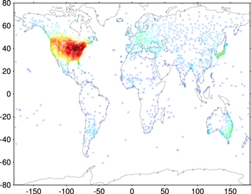
Figure 1. Locations of GHCN stations used in this study. 'Hotter' marker colors correspond to locally higher station density.
Download figure:
Standard image High-resolution image2.2. Climatology construction methods
We assumed that the yearly time series of temperature for a given calendar month T(t) can be represented as the sum of a smooth trend component  and a zero-mean high-frequency component
  [13]:
[13]:

Using this framework, our goal was to estimate a probability distribution for T at a given year tf, given observations from previous years. We took the expectation of  , or Tf for short, to be equal to
  thus neglecting any information that might be available, particularly for short lead times, about the high-frequency component
  which various methods of seasonal forecasting attempt to estimate [10, 14–16]. The probability distribution of
  therefore includes uncertainty due to
  which will be the same for all the methods considered here, as well as uncertainty in estimating
  from available previous observations.
A common class of methods for estimating Tf is the moving average  where the estimate is the average value of T over the previous n years for which observations are available. Previous comparisons focusing on the United States [6, 7] found that
  minimizes mean square error for seasonal temperature series over recent years. The 30-year standard WMO averaging corresponds to
  (30) (although here we update the averaging period annually rather than only every 10–30 years as is typically done for climatological standard normals), whereas with a value of n at least equal to the observational record length
  reduces to the average of all previous observations, which would be the optimal estimate of the expected value in a stationary climate. Here we considered values of n equal to 5, 10, 15, 30, 60, and 90 years.
A second method considered for estimating Tf is the exponentially weighted moving average  . Unlike the moving average, this uses all the past observations T but gives more weighting to the more recent observations, which offers theoretically optimal predictions if the trend follows a random walk [17]. The behavior of the exponentially weighted moving average depends on its e-folding weighting timescale
  Here we considered timescales τ equal to 5, 10, 15, 30, 60, and 90 years, allowing direct comparison with the simple moving average results. Large τ correspond to weighting all past observations equally, whereas small τ correspond to giving significant weights only to the most recent observations.
A third method considered is the hinge fit [2]. This uses only observations since 1940 and estimates Tf by piecewise linear regression with a break point at 1975. At the break point, the fitted temperature is continuous, but its first derivative is discontinuous. One version of the hinge fit ( ) assumes that
  was constant between 1940 and 1975, whereas a second version (
 ) fits a slope for
  between 1940 and 1975 as well as after 1975 [7].
We also tested several more complex methods, including polynomial fits, linear regression using atmospheric CO2 concentration as a predictor [18], and a smoothing cubic spline fit to all previous observations with smoothing parameter p [19, chapter XIV]. Since in our preliminary tests these methods did not outperform the simpler methods just described for monthly temperature prediction at individual stations, we do not consider them further here.
2.3. Forecast probability distributions
Each of the above methods, for a given choice of parameter (e.g., n or τ), estimates  as a linear combination of the observed
  If
If  actually follows the assumed linear model and the
  terms are independent identically distributed Gaussian variables, the predictive distribution of Tf given the observations T can be calculated as a Student t distribution centered at the estimated
  giving the required probability distribution for the expected temperature at tf [20].
The t distribution with mean  scale parameter
  and ν degrees of freedom is given by
For MA(n), μ is simply the mean of the past n observations, σ is the sample standard deviation of the observations, and ν is equal to 
For EW(τ), define  quantifying the relative magnitude of the trend compared with interannual variability [21]. Then we get


where  is the
  vector of observed past temperatures,
  is an
is an  vector of ones, and
  is the inverse of the model covariance matrix
  defined as

with  the
the  identity matrix and
  the
the  matrix with elements

where tf is the forecast time and ti are the n past observation times [21].
For a general linear regression such as the hinge fit, define  to be the
  matrix of predictor values at the observation times and
  to be the
  vector of predictor values at the forecast time
  Then
Then


where k is the number of regression coefficients (2 for  and 3 for
  ).
).
2.4. Bias–variance trade-off and empirical adjustment
Bias–variance trade-off is characteristic of a wide variety of inference problems and methods [22, 23]. The temperature trend at tf is best estimated by using recent observations, but these observations are not numerous enough to confidently separate the trend from interannual variability subsumed under  On the other hand, averaging observations over a long period will reduce the influence of
  but also obscure recent climate changes. This trade-off can be studied quantitatively with a bias–variance decomposition of mean square hindcast error (MSE):
where  denotes the predicted expectation, y is the actual value, and
  denotes averaging over hindcasts. Figure 2 (see [24] for a somewhat similar concept) shows these bias and variance components with the GHCN data for
  and
and  with averaging timescales
  ranging from 5 to 90 years. Small
  corresponds to little bias but high variance, whereas high
  leads to reduced variance but mean bias of
  K since current conditions are substantially warmer than the average of a long series of past observations. MSE is thus minimized at intermediate
  of
of  years. The
  curve is slightly below and to the left of the
  curve on this plot, indicating that
  offers improved bias–variance characteristics compared with what is possible with
  On the other hand, the hinge fits offer low bias but mean variance higher than any of the
  or
or  cases (figure 2).

Figure 2. Bias and variance for moving average (MA) and exponentially weighted moving average (EW) hindcasts with different averaging timescales, as well as for hinge fit (HF) hindcasts. The EW and MA markers correspond to timescales of 5, 10, 15, 30, 60, and 90 years, with larger markers used for longer timescales. Empirical adjustment for bias reduces the MA and EW bias magnitudes while having little impact on variance, resulting in more accurate hindcasts. Dashed curves are contours of constant root mean square error, with a contour interval of 0.05 K. The bias and variance are averages over all available GHCN stations and months for the last 30 years.
Download figure:
Standard image High-resolution imageIt is possible to sharply reduce the bias by consideration of the global mean warming trend. This is because the amplitude of the interannual variability is much smaller for global mean temperatures than for individual stations, so it is possible to estimate the global trend accurately. We estimated the global trend by spline smoothing of a global mean temperature series, with the smoothing parameter value p chosen to minimize the corrected Akaike information criterion [25, 26]. Accurate estimates of the expected bias, for example, for an  or
or  estimate, can be obtained using the less-variable global series, and this bias can then be subtracted from the
  or
or  expectation μ for each station. As expected, this bias is greater for longer averaging timescales and shows some variability and a general increase in magnitude over time, particularly for longer τ (figure 3). The MA case is similar, with an averaging timescale even as short as 15 years [7] having a consistent, albeit modest
  , negative bias because it does not fully capture recent warming.
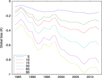
Figure 3. Bias of exponentially weighted moving average estimators with different  estimated for each hindcast year using a spline fit to global mean temperature. For any given year, longer averaging timescale τ is associated with greater (more negative) bias.
Download figure:
Standard image High-resolution imageAdjusting the forecast probability distributions by an additive factor as shown in figure 3 does greatly reduce the bias term even for large τ ('adjusted' curves in figure 2). After bias adjustment, the minimum hindcast root mean square error decreases ∼2% from ∼1.92 K to ∼1.89 K, and this minimum is reached at  years (figure 3).
An example of the hindcast expected values for  with and without bias adjustment is shown in figure 4(a). The unadjusted
  method has a clear low bias, which adjustment largely removed through translating the probability distribution (i.e., changing the mean μ) by 0.16 K for 1984, increasing to 0.39 K by 2013 (see figure 3). The adjusted
  probabilistic hindcasts (figure 4(b)) show the large effect of the warming trend particularly on the expected frequencies of temperatures at the hot and cold extremes of the distributions.
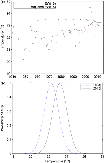
Figure 4. (a) Example observation and hindcast series—June temperatures from Nagasaki, Japan. (b) Hindcast probability distributions as of 1984 and 2013. See text for details of the hindcasts.
Download figure:
Standard image High-resolution image2.5. Climatology skill metrics
MSE (or its square root, RMSE) and its bias and variance components are useful and widely employed for evaluating the skill of point estimates of climatology. Additional metrics are needed, however, to evaluate the skill of probabilistic climatologies. The skill of a probabilistic forecast may be evaluated by how probable the actual outcomes are in the forecast. This can be quantified with the mean negative log likelihood (NLL):

where p is the hindcast probability distribution and y is the observed temperature. The NLL values for different forecast methods have units of information (bits or nats, depending on the base of the logarithm taken—here we take natural logarithms) and can be related to the methods' ability to reduce uncertainty in a decision-making framework [10, 27–29]. NLL is a strictly proper forecast-evaluation skill score which is sensitive to both the mean of the forecast distribution and its variance [30, 31].
Particularly for assessing the likelihood of extreme events, it is also important that the method produce probability distributions that are consistent with the observed values. This can be assessed graphically by plotting the histogram of the hindcast cumulative distribution function at the observed temperature (known as the rank verification histogram [32]), which should approximate the uniform distribution, and numerically by calculating the Kolmogorov-Smirnov statistic Dn for the maximum deviation of the empirical cumulative distribution from the standard uniform distribution. Dn ranges between 0 and 1, and for n independent trials and a well-calibrated forecast method should tend to zero as  [33]. In practice we cannot compute exactly how small we expect this statistic to be under the assumptions of each method because this depends on the correlation of temperature data across different stations and months [32], which is difficult to estimate; still, lower values of this statistic generally indicate better-performing probabilistic forecast methods.
Here we averaged metrics such as MSE, NLL, and Dn across years and stations to produce global skill measures. The same metrics could also be averaged for spatiotemporal subsets in order to study, for example, whether the ranking of methods is consistent across regions or seasons.
3. Results
3.1. Hindcast performance across methods
Without adjustment, the MA and EW methods all tend to give temperature hindcasts that are biased cold, meaning that they underestimate the warming seen (table 1). Reducing n in the MA method or τ in the EW method reduces the magnitude of this bias, but at the cost of higher variance. RMSE, which combines bias and variance, is lowest for  , with
  close behind. The information measure NLL gives the same ranking. The negative bias means that EW and MA hindcasts present cold conditions as more probable, and hot conditions as less probable, than was actually the case (figure 5(a)), a mismatch that gives values of the Kolmogorov-Smirnov statistic around 0.07–0.10 for the most skillful EW and MA variants. The hinge fit methods have little bias (
 0.1 K) and good Kolmogorov-Smirnov statistics of under 0.01, but higher variance, so their overall performance as measured by RMSE and NLL is worse than that of EW and MA methods (table 1).
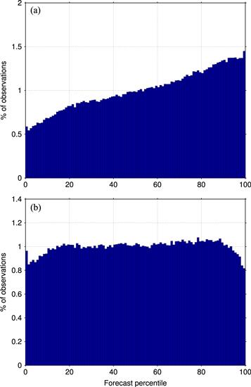
Figure 5. Frequency distribution of observed values as percentiles of the hindcast probability distribution for the exponentially weighted moving average  method (a) without bias adjustment, (b) with bias adjustment. For a well-calibrated forecast, this histogram should be flat.
Download figure:
Standard image High-resolution imageTable 1. Temperature hindcast skill metrics for methods without additional bias adjustment. For all metrics shown, values closer to zero indicate a more skillful method. See the text for details of the methods compared. RMSE = root mean square error; NLL = mean negative log likelihood; Dn = Kolmogorov-Smirnov statistic.
| Method | Bias (K) |
 (K) (K) |
RMSE (K) | NLL (nats) | Dn (%) |
|---|---|---|---|---|---|
| MA(5) | −0.089 | 2.023 | 2.025 | 2.273 | 6.22 |
| MA(10) | −0.174 | 1.934 | 1.942 | 1.974 | 5.74 |
| MA(15) | −0.256 | 1.908 | 1.925 | 1.928 | 7.42 |
| MA(30) | −0.433 | 1.895 | 1.944 | 1.926 | 11.53 |
| MA(60) | −0.509 | 1.901 | 1.968 | 1.947 | 13.42 |
| MA(90) | −0.571 | 1.910 | 1.993 | 1.966 | 14.80 |
| EW(5) | −0.159 | 1.937 | 1.944 | 1.894 | 4.23 |

|
−0.274 | 1.896 | 1.916 | 1.885 | 7.28 |
| EW(15) | −0.349 | 1.886 | 1.918 | 1.893 | 9.26 |
| EW(30) | −0.465 | 1.886 | 1.943 | 1.921 | 12.22 |
| EW(60) | −0.547 | 1.900 | 1.977 | 1.951 | 14.15 |
| EW(90) | −0.573 | 1.908 | 1.992 | 1.962 | 14.76 |

|
−0.014 | 2.042 | 2.042 | 1.940 | 0.44 |

|
+0.033 | 2.044 | 2.044 | 1.940 | 0.69 |
After bias adjustment, the MA and EW methods have greatly reduced mean bias, generally under 0.1 K regardless of the exact parameter values used, whereas the hindcast variance is little affected (table 2).  is now the best performer as measured by NLL, with a decrease of some 2% in RMSE and 0.04 bits in NLL due to bias adjustment, followed by
  and
and  .
.  ranks best in terms of RMSE. (It is expected that bias adjustment will tend to increase the optimal values of the averaging timescale n or
  since now bias is a smaller contributor to the error, allowing us to take advantage of the reduced variance afforded by a longer averaging time.) The Kolmogorov-Smirnov statistic for these methods is around 0.01, indicating a much better calibrated probabilistic hindcast that is comparable in quality to the hinge fit results. This improvement can be clearly seen in rank verification histograms (figure 5(b)).
Table 2. Temperature hindcast skill metrics. Same as table 1, but with global bias adjustment.
| Method | Bias (K) |
 (K) (K) |
RMSE (K) | NLL (nats) | Dn (%) |
|---|---|---|---|---|---|
| MA(5) | −0.025 | 2.021 | 2.022 | 2.269 | 5.16 |
| MA(10) | −0.047 | 1.935 | 1.936 | 1.970 | 2.67 |
| MA(15) | −0.063 | 1.911 | 1.912 | 1.916 | 2.23 |
| MA(30) | −0.079 | 1.897 | 1.898 | 1.886 | 1.69 |
| MA(60) | −0.055 | 1.899 | 1.899 | 1.883 | 0.92 |
| MA(90) | −0.044 | 1.907 | 1.908 | 1.890 | 0.47 |
| EW(5) | −0.032 | 1.939 | 1.939 | 1.889 | 0.91 |

|
−0.047 | 1.899 | 1.900 | 1.870 | 1.04 |
| EW(15) | −0.052 | 1.889 | 1.889 | 1.867 | 1.04 |
| EW(30) | −0.038 | 1.887 | 1.888 | 1.871 | 0.79 |
| EW(60) | +0.044 | 1.899 | 1.900 | 1.886 | 2.20 |
| EW(90) | +0.114 | 1.906 | 1.909 | 1.899 | 4.14 |

|
−0.019 | 2.043 | 2.043 | 1.942 | 0.52 |

|
−0.007 | 2.045 | 2.045 | 1.940 | 0.47 |
To test the sensitivity of our results to the geographic distribution of stations used, we also calculated RMSE and NLL global skill metrics with an alternative averaging procedure where stations that were close together were weighted less, thus reducing the influence of dense clusters of observations, such as those in the United States. The weight assigned to each station was proportional to the reciprocal of the local station density estimated by an exponential density kernel with a length scale of 3 (see figure 1). The rankings of the methods did not change greatly under this weighting, but the optimal averaging timescale tended to be somewhat shorter than when stations were weighted equally (tables 3 and 4): for example, the method with lowest RMSE after bias adjustment was
  , and the method with lowest NLL was
  .
.
Table 3. Temperature hindcast skill metrics for methods without additional bias adjustment. For all metrics shown, values closer to zero indicate a more skillful method. Same as table 1 except that here the averaging of metrics across stations downweights stations that are close together. RMSE = root mean square error; NLL = mean negative log likelihood.
| Method | Bias (K) |
 (K) (K) |
RMSE (K) | NLL (nats) |
|---|---|---|---|---|
| MA(5) | −0.078 | 1.856 | 1.858 | 2.023 |
| MA(10) | −0.159 | 1.775 | 1.783 | 1.706 |
| MA(15) | −0.244 | 1.765 | 1.782 | 1.670 |
| MA(30) | −0.430 | 1.756 | 1.808 | 1.696 |
| MA(60) | −0.585 | 1.762 | 1.856 | 1.776 |
| MA(90) | −0.643 | 1.766 | 1.880 | 1.806 |
| EW(5) | −0.147 | 1.780 | 1.786 | 1.612 |

|
−0.269 | 1.747 | 1.768 | 1.622 |
| EW(15) | −0.357 | 1.741 | 1.777 | 1.648 |
| EW(30) | −0.504 | 1.745 | 1.816 | 1.716 |
| EW(60) | −0.606 | 1.758 | 1.859 | 1.776 |
| EW(90) | −0.638 | 1.764 | 1.876 | 1.796 |

|
+0.050 | 1.884 | 1.885 | 1.671 |

|
+0.054 | 1.884 | 1.884 | 1.661 |
Table 4. Temperature hindcast skill metrics for methods. Same as table 3, but with global bias adjustment.
| Method | Bias (K) |
 (K) (K) |
RMSE (K) | NLL (nats) |
|---|---|---|---|---|
| MA(5) | −0.009 | 1.856 | 1.856 | 2.024 |
| MA(10) | −0.032 | 1.776 | 1.776 | 1.698 |
| MA(15) | −0.048 | 1.765 | 1.766 | 1.654 |
| MA(30) | −0.067 | 1.755 | 1.756 | 1.633 |
| MA(60) | −0.104 | 1.758 | 1.761 | 1.647 |
| MA(90) | −0.089 | 1.763 | 1.765 | 1.655 |
| EW(5) | −0.016 | 1.780 | 1.780 | 1.606 |

|
−0.034 | 1.748 | 1.748 | 1.598 |
| EW(15) | −0.049 | 1.741 | 1.742 | 1.603 |
| EW(30) | −0.059 | 1.744 | 1.744 | 1.622 |
| EW(60) | +0.010 | 1.756 | 1.756 | 1.653 |
| EW(90) | +0.078 | 1.762 | 1.764 | 1.677 |

|
+0.048 | 1.884 | 1.884 | 1.672 |

|
+0.017 | 1.883 | 1.884 | 1.660 |
We conducted similar analyses using mean-monthly daily minimum and maximum temperatures from GHCN rather than mean temperatures. These gave qualitatively similar results to those seen for mean temperatures, including a bias–variance trade-off for the EW and MA methods and high error variance for the hinge fit methods. In these two cases bias-adjusted  had the best overall performance as measured by both RMSE and NLL.
3.2. Changing frequency of monthly temperature extremes
The bias-adjusted probabilistic EW(15) hindcasts can be used to estimate how monthly temperature quantiles have shifted over time. For example, over the GHCN stations, the 1st percentile monthly temperature value in 1984 (a one-in-100-year cold event) became on average the 0.32 percentile by 2013, i.e., the recurrence interval lengthened to over 300 years. The 99th percentile monthly temperature value in 1984 (a one-in-100-year hot event) became on average the 95.3 percentile by 2013, i.e., the recurrence interval dropped to under 25 years. Thus, extreme hot episodes have become much more likely in just a few decades, whereas extreme cold episodes have become less likely. For the less extreme 10 and 90 percentiles, the corresponding shifts are to 4.2 and 76.0, so the frequency of cold months has dropped whereas the frequency of hot months has increased by more than a factor of 2. These global average changes were fairly robust to the specific climatology estimation method used. The spatial distribution of the estimated 2013 frequencies of the onetime 100-year events (figure 6) suggests that the changes may tend to be greater in the tropics and in areas with maritime climates, where interannual variability is smaller compared with the warming trend [34].

Figure 6. Estimated percentiles of (a) extreme hot and (b) extreme cold months (percentiles 99 and 1 of the 1984 distribution) as of 2013. Extreme hot months have become more common (so that they are well below the 99th percentile of the present-day distribution), whereas extreme cold months have become less common (so that they are well below the present-day 1st percentile). Station values have been averaged on a  grid for display.
Download figure:
Standard image High-resolution image
4. Discussion
The probabilistic climatology update methods described here have a number of potential applications, from assessing the time-evolving risk of ecologically relevant extremes [35] to preparedness by utilities and municipalities for cold and hot conditions [7]. To facilitate such applications, free software implementations of the methods described are available at http://bitbucket.org/niryk/logocline. Our approach enables estimating any desired quantiles of the current/near-future temperature probability distribution wherever there are high-quality time series of past observations without use of numerical climate models. It thus complements related avenues of investigation, such as attribution of specific heat waves to anthropogenic global warming [36, 37], the changing relative frequencies of new record high versus record low temperatures [38–40], and assessments based on climate models of the future risk for extreme conditions [34, 41–43].
A number of directions for possible improvement of these time-evolving probabilistic climatologies could be pursued. The exponentially weighted moving average with global bias adjustment and a timescale of 15 years has been shown to be a good choice compared with the other methods considered for estimating current temperature expectations over the current weather station network. More specifically, the optimum timescale after bias adjustment seems to be in the range of 10–30 years, with the exact value depending somewhat on the skill metric chosen and on the geographic distribution of stations considered. Methods could be considered for adaptively choosing the timescale based on available data [21]. The global bias adjustment might be improved by considering regional and seasonal variations in the rate of warming to the extent that these can be reliably deduced from observational records; this could be implemented as hierarchical Bayesian estimation, with hyperparameters controlling the degree to which bias correction pools data across space and time [44, 45].
Note that the absolute differences between methods in some skill metrics such as RMSE are small—no more than a few percent (figure 2). This is simply because the interannual variability in station monthly temperatures, which we do not attempt to predict as part of constructing updated climate normals, tends to be large compared with the climate trend seen over the last few decades. Where the climate trend signal is larger, for example, for regional to global average temperatures and for longer-term averages, the relative impact of updating climate normals would be expected to increase. As well, the information offered by updated climate normals can serve as the base for probabilistic seasonal forecasts that better capture year-to-year temperature variability using information about persistent forcings such as the Southern Oscillation [10, 46].
Although the exponentially weighted moving average with global bias adjustment and the assumption that interannual variability is normally distributed produced probabilistic forecasts that were fairly well calibrated, there were some 10–20% more hindcasts for extreme cold and heat (bottom and top few percentiles) than actually observed events (figure 5(b)). This may be attributed to decadal variability (with the last 30 years having fewer extremes than average); indicate a slight reduction in temperature variance through time (which is in fact predicted by climate models, although not yet conclusively seen in observations [47–50]); or be due to the distribution of monthly temperatures actually having slightly narrower tails than a normal distribution with the same variance. Daily temperature series show some asymmetry compared with a normal distribution, suggesting that even for monthly temperatures, it may be possible to improve the estimated probabilities of extreme values by adopting a more general probability distribution such as the skew-normal [51, 52].
5. Conclusion
We have demonstrated time-evolving probabilistic temperature climatologies that can be used to assess the chance that temperatures will fall within any prescribed range over an upcoming month. Such probabilistic climatologies illustrate the rate of change in the frequency of extreme conditions.
Acknowledgments
The authors gratefully acknowledge support from NOAA under grants NA11SEC4810004 and NA12OAR4310084. All statements made are the views of the authors and not the opinions of the funding agency or the US government.