

Abstract
We analyzed a dataset from an experiment of an earth system model of intermediate complexity, focusing on the change in transient climate response to cumulative carbon emissions (TCRE) after atmospheric CO2 concentration was stabilized in the Representative Concentration Pathway (RCP) 4.5. We estimated the TCRE in 2005 at 0.3–2.4 K/TtC for an unconstrained case and 1.1–1.7 K/TtC when constrained with historical and present-day observational data, the latter result being consistent with other studies. The range of TCRE increased when the increase of CO2 concentration was moderated and then stabilized. This is because the larger (smaller) TCRE members yield even greater (less) TCRE. An additional experiment to assess the equilibrium state revealed significant changes in temperature and cumulative carbon emissions after 2300. We also found that variation of land carbon uptake is significant to the total allowable carbon emissions and subsequent change of the TCRE. Additionally, in our experiment, we revealed that equilibrium climate sensitivity (ECS), one of the 12 parameters perturbed in the ensemble experiment, has a strong positive relationship with the TCRE at the beginning of the stabilization and its subsequent change. We confirmed that for participant models in the Coupled Model Intercomparison Project Phase 5, ECS has a strong positive relationship with TCRE. For models using similar experimental settings, there is a positive relationship with TCRE for the start of the period of stabilization in CO2 concentration, and rate of change after stabilization. The results of this study are influential regarding the total allowable carbon emissions calculated from the TCRE and the temperature increase set as the mitigation target.
Export citation and abstract BibTeX RIS

Content from this work may be used under the terms of the Creative Commons Attribution 3.0 licence. Any further distribution of this work must maintain attribution to the author(s) and the title of the work, journal citation and DOI.
1. Introduction
The transient climate response to cumulative carbon emissions (TCRE) is defined as the global mean surface temperature change per 1000 GtC (=1TtC) anthropogenic CO2 emissions, and the proportionality is assumed constant only while the temperature is increasing (Collins et al 2013). This parameter (and its constancy) is very helpful in addressing future carbon emission pathways because we can estimate the total permissible amount of future CO2 emissions for a given climate stabilization target of temperature anomaly and, because the temperature increase is scenario-independent, we can determine the pathway based solely on economic feasibility.
Current uncertainty in the estimation of the TCRE is considerable. Allen et al (2009) obtained a range of 1.4–2.5 K/TtC using ensemble simulations of simple climate–carbon-cycle models constrained by observations and projections from more comprehensive models with broad-ranging CO2 emission pathways. Matthews et al (2009) obtained a range of 1.0–2.1 K/TtC based on results from Coupled Climate Carbon Cycle Model Intercomparison Project (C4MIP) models, including seven state-of-the-art earth system models (ESMs) and four ESMs of intermediate complexity (EMICs). Gillett et al (2013) obtained a range of 0.7–2.0 °C/TtC from results of the Coupled Model Intercomparison Project Phase 5 (CMIP5).
Although not included in TCRE focusing on transient response, there can be slight warming after the cessation of carbon emissions. For that, the peak response to cumulative emissions (PRCE) was defined using a maximum temperature (Bindoff et al 2013). PRCE is greater than TCRE when there is significant delay in the earth system temperature response to an increase of atmospheric CO2; otherwise, the two are nearly identical (Collins et al 2013). It is more difficult to constrain PRCE than TCRE; ranges of 1.3–3.9 K/TtC (Allen et al 2009) and 1.1–2.7 K/TtC (Meinshausen et al 2009) have been reported. The increase in the estimated range by Allen et al (2009), from 1.1 K/TtC for TCRE to 2.6 K/TtC for PRCE, implies that the earth system behaviour after the cessation of CO2 emissions amplifies the uncertainty in the ratio of temperature to cumulative carbon emissions.
Frölicher et al (2014) argued that contrasting behaviours after the cessation of carbon emissions are caused by differences in ocean heat efficacy, determined by ocean circulations and the resultant geographic distribution of ocean heat uptake (OHU). In further discussion on the temperature change after the cessation of CO2 emissions, Frölicher and Paynter (2015) defined the equilibrium climate response to cumulative carbon emissions (ECRE) and the multi-millennial climate response to cumulative carbon emissions (MCRE). These metrics are calculated similarly to TCRE but instead, use the temperature when OHU is zero (ECRE), or the temperature when the exchange of carbon between the atmosphere and global ocean ceases (MCRE).
In assessing the temperature change after the cessation of CO2 emissions, we should also note that the treatment of both aerosol and non-CO2 greenhouse gas forcing could have significant impact. The effects of the removal of both aerosol and non-CO2 greenhouse gas forcing are largely negated when best-estimate aerosol forcing is used; however, this cancellation is tentative because each of the two forcings is large and there is significant uncertainty regarding historical aerosol forcing (Matthews and Zickfeld 2012).
These uncertainties in TCRE and its derivative metrics are serious problems when applying their values to estimations of how much CO2 could be emitted for a given temperature target. The Fifth Assessment Report of the IPCC (2013) showed a slight decrease in TCRE after the atmospheric pCO2 stabilized in the Representative Concentration Pathway (RCP) 2.6 and RCP4.5 scenarios. However, Hajima et al (2012) reported some increase in TCRE using the MIROC-ESM (with large climate sensitivity of 4.7 K), implying significant model dependence of TCRE during the final parts, i.e. when pCO2 is stabilized or decreasing, of the two scenarios. Using a large perturbed parameter ensemble and a type of EMIC, Tachiiri et al (2013) showed that the TCRE ensemble mean remained constant throughout an experiment with the RCP2.6 and RCP4.5 scenarios and during the transition from RCP4.5 to RCP2.6.
In the present study, which focused on the uncertainty of TCRE after stabilization, we reanalyzed the results of Tachiiri et al (2013) and performed an experiment to assess the equilibrium states. By analyzing large ensemble datasets, we filled the gap not covered by the limited number of comprehensive models.
2. Method
The experiment (Tachiiri et al 2013) was performed using an EMIC called the Japan Uncertainty Modelling Project—Loosely Coupled Model (JUMP-LCM; Tachiiri et al 2010), which has a two-dimensional energy–moisture balance atmosphere, coupled with an ocean general circulation model. In addition, a process-based land ecosystem model is 'loosely coupled'. We took the global mean temperature from the EMIC and found a year with a corresponding temperature, from a run of a general circulation model (GCM, MIROC3.2) with a 1% per year (1 ppa) increase in CO2 concentration, and used that to drive the land component. In the experiment using an ensemble of 512 members, 12 parameters, both physical and biogeochemical, were perturbed using Latin hyper-cube sampling. The resultant ranges both in the linear transient climate sensitivity (α in Friedlingstein et al 2006) and in the sensitivities of land and ocean carbon storage to atmospheric CO2 concentration change (β) and temperature change (γ) were as close as possible to those of the C4MIP models (β and γ were tuned separately for the land and ocean, respectively).
The perturbed parameters were the equilibrium climate sensitivity (ECS), vertical and horizontal diffusivities of the ocean, Gent–McWilliams thickness parameter (Gent and McWilliams 1990), magnitude of freshwater flux adjustment, wind speed used in marine CO2 uptake, maximum photosynthetic rate (of land), specific leaf area, minimum temperature for photosynthesis (of land), coefficient for temperature dependence of plant respiration, temperature dependence of soil respiration, and total aerosol forcing (considered as radiative forcing relative to the level of 1850). These included some EMIC-specific parameters. First, ECS is not easily controllable in state-of-the-art climatic models (ESMs or global circulation models), but is possible in EMICs with an energy-balance atmosphere. In addition, the magnitude of freshwater flux adjustment is a parameter supporting inter-ocean freshwater flux, which is not needed in many cases for more comprehensive climatic models. The wind speed used in marine CO2 uptake, which is the only perturbed parameter related to the marine carbon cycle, is EMIC-specific. Because wind speeds calculated in the EMIC do not represent observed fields well, a constant value is used in calculating the ocean carbon uptake, although we perturbed that constant in the experiment. In addition, the scale of aerosol forcing, which is not a model parameter but considers the uncertainty of the forcing, was also perturbed and found to have significant impact, particularly on temperature.
Among the three scenarios used in Tachiiri et al (2013), we focused on RCP4.5 and its extension to 2300 to investigate the TCRE change after atmospheric CO2 concentration was stabilized. After the experiments, each ensemble member was weighted with the representability of historical trends of global mean surface air temperature, historical trends of ocean heat content for the depth of 0–700 m, historical fossil fuel emissions, terrestrial net primary production, Atlantic meridional overturning circulation, and present air surface temperature, sea temperature, and sea salinity. The results obtained before and after this process were denoted the unconstrained and constrained cases, respectively.
We also performed an additional experiment, running each ensemble member to the equilibrium state at an atmospheric CO2 concentration of 543 ppm (the target in RCP4.5). Because the JUMP-LCM is a loosely coupled model, this was done separately for the atmosphere–ocean and land, as follows. First, we ran the coupled atmosphere–ocean part for 3000 years to equilibrate the atmosphere and ocean, and we used the difference between the equilibrium temperatures at 285 and 543 ppm to find a year with the corresponding temperature anomaly from the MIROC3.2 output with the 1 ppa scenario to run the land ecosystem model. Because we used data for the same year 2000 times to equilibrate the land, the effect of the interannual variability of climatic conditions on land carbon storage was not considered. Among the 512 ensemble members, the difference in equilibrium temperature between the two CO2 concentration levels was outside the range of the 150-year-run dataset for only four members. In such cases, data of the last (150th) year were used to run the land ecosystem model. Because this occurred for only a small number of members, and the curtailed temperatures were not large (0.05–0.25 K), we believed that the effect of this process was limited, particularly on the statistics of the data. Another difference from the previous experiment with RCP4.5 was that non-CO2 (including aerosol) forcing was switched off throughout this run.
Using the results of the above experiments, we analyzed both the TCRE uncertainty after the atmospheric CO2 concentration was stabilized and the contributions of the various parameters to that uncertainty. Here, we calculated the TCRE as follows:
where ΔTCO2 is the CO2-induced warming estimated using the temperature anomaly (ΔT), total (RFall) and CO2-induced (RFCO2) radiative forcing (Meinshausen et al 2011) as:

and CA, CO, and CL are the contents of carbon in the atmosphere, ocean, and land, respectively. The term −γ(ΔT—ΔTCO2) in the denominator of equation (1) is a corrective term used to estimate the difference in Δ(CO + CL) between cases in which the temperature anomaly is ΔT and ΔTCO2. Here, γ (sensitivity of total land and ocean carbon storage to temperature) is estimated as a linear function of ΔT from a small ensemble experiment at the tuning stage. LUE is the CO2 emission from land use (Clarke et al 2007, Smith and Wigley 2006, Wise et al 2009). In the analysis, we note that TCRE is determined by a combination of physical and biogeochemical sensitivities. Based on Friedlingstein et al (2006), such sensitivities determining the response of the earth system to changing CO2 concentration are classified as the linear transient climate response (α), concentration-carbon (β) and climate-carbon (γ) feedback of the land and ocean. Using α, β, γ, and CA, the cumulative carbon emission (CE) is expressed as follows (Gregory et al 2009):
Thus, from this we obtain

By decomposing β and γ into land (βL, γL) and ocean (βO, γO), we obtain
Because in all the ESMs, γL is larger and more negative than γO (and βL and βO are similar; Arora et al 2013), it is usual that ocean carbon uptake is greater than land carbon uptake.
To indicate the climate response to cumulative carbon emissions in the equilibrium state, we use ECRE, following Frölicher and Paynter (2015), noting that in this study, unlike their experiment, it was difficult to distinguish ECRE from MCRE.
3. Results and discussion
In the analyzed data, the estimated TCRE for 2005 (average of 2001–2010) was 0.3–2.4 K/TtC (5–95% range) for the unconstrained case and 1.1–1.7 K/TtC for the constrained case. The latter range is slightly narrower but overall, they are consistent with existing works. However, as the temporal changes in TCRE (5th, 16th, 50th, 84th and 95th percentiles; figure 1) show, the TCRE range expanded in the latter half of the experiment. In the unconstrained case, the upper bound of the 90% (5–95%) range increased, whereas the lower bound gradually decreased, expanding the 90% range (figure 1(a)). This was even more significant for the constrained case (figure 1(b)), in which the range of the 90% was well constrained (about 0.6 K/TtC) in the early 21st century, but increased to about 2.9 K/TtC by 2300.
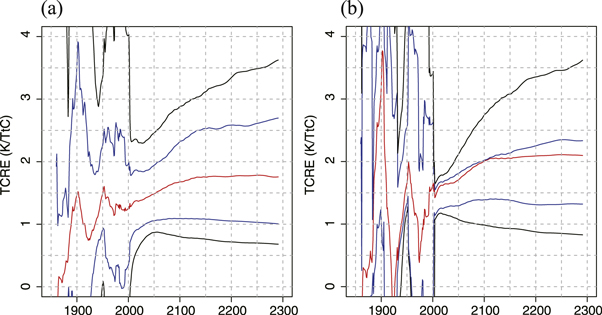
Figure 1. Temporal change in range of uncertainty of TCRE for RCP4.5: (a) unconstrained and (b) constrained cases. Red: median, blue: 16th and 84th percentiles, black: 5th and 95th percentiles. Data source: Tachiiri et al (2013). TCRE is calculated using equation (1). Twenty-year averages are presented.
Download figure:
Standard image High-resolution imageTo investigate the reason why the uncertainty increased after stabilization, we first plotted the temporal change of the temperature anomaly and cumulative carbon emission (CE) for each member (figure 2(a)). In figure 2(a), the slope of temperature increase versus CE (or TCRE) before stabilization is relatively stable, but after stabilization, the ensemble members with small TCRE had stable temperatures and increasing CE, which resulted in decreased TCRE. Conversely, ensemble members with large TCRE had increasing temperature and stable or decreasing CE; thereby increasing the TCRE. For some members beyond the 5%–95% range, i.e., very low consistency with the observations, TCRE ultimately became negative because CE became negative. Such members result from the exploration of a wide range of model parameters and are unlikely to be realistic possibilities. Expansion of the range of uncertainty in TCRE shows that it is difficult to constrain TCRE after stabilization using observed data from the period of CO2 increase.

Figure 2. (a) All 512 members. Pink (1850–2115, i.e., before CO2 concentration is nearly stabilized) and red (2115–2300) curves represent the ensemble members within the 5–95% TCRE range for each year (after the constraint). Grey and black curves are the same but for those beyond the 5–95% TCRE range for each year. (b) After grouping based on average TCRE in 2111–2120: <1.0 (black), 1.0–1.5 (red), 1.5–2.0 (green), 2.0–2.5 (blue), 2.5–3.0 (cyan), 3.0–3.5 (magenta), and >3.5 (grey) K/TtC (years before 2010 are not presented because they demonstrated too much fluctuation). The solid and dotted lines present 1850–2115 and 2115–2300, respectively. Points at years 2100 and 2200 in curves are connected by dashed black lines to show their relative positions in those years. Open circles depict equilibrium states (after 3000-year run for atmosphere and ocean and 2000-year run for land). Data source, except for open circles in (b), was Tachiiri et al (2013). Plotted are the numerator and denominator of equation (1).
Download figure:
Standard image High-resolution imageFigure 2(b) is similar to figure 2(a), but it presents the results after all the ensemble members were combined into seven groups based on average TCRE values in 2111–2120 (when CO2 concentration was nearly stabilized), with thresholds of 1.0, 1.5, 2.0, 2.5, 3.0 and 3.5 K/TtC.
Ensemble members with small TCRE move right (i.e., TCRE is decreasing) in the figure after stabilization, whereas those with large TCRE move up or left (i.e., increasing temperature with stable or decreasing CE). Another important point presented in figure 2(b) is that all groups move toward the point of equilibrium, but that significant differences remain between 2300 and equilibrium (indicated by the open circles) in temperature and cumulative emissions.
The variation in trajectories after stabilization, for groups with different TCRE, can be attributed partially to the difference in relationship between levels of equilibration in temperature and carbon. That is, in the groups with small TCRE values (black curve in figure 2(b)), temperature does not rise after 2110s, whereas CE increases after that. In other words, temperature almost achieved the equilibrium state in 2110s, but carbon remained far from equilibrium and it required a longer time to equilibrate. In contrast, for the group with large TCRE (grey curve in figure 2(b)), temperature remained far from equilibrium, whereas carbon was near equilibrium in comparison with the small TCRE group, although it remained some distance from that equilibrium.
Figure 3 shows the contributions by land and ocean to CE of each member. For the ocean (figure 3(a)), the slope of the temperature anomaly versus the change in carbon storage (or cumulative carbon uptake) decreased after stabilization for all members. However, for land (figure 3(b)), the slope decreased for only a limited number of members; for most, carbon storage was stable or it declined with temperature increase. It is apparent that the land was the main contributor to the change characteristics of TCRE (shown in figure 2) for members with large TCRE.
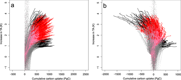
Figure 3. Modelled time-evolving relationships between air temperature change (CO2-induced) and cumulative land/ocean carbon uptakes for each ensemble member and RCP4.5: (a) ocean and (b) land. Pink (1850–2115, before CO2 concentration is nearly stabilized) and red (after that) curves represent the ensemble members within the 5–95% TCRE range for each year after constraints. Grey and black curves are the same but for those beyond the 5–95% TCRE range for each year.
Download figure:
Standard image High-resolution imageIt appears from figure 2(b) that two groups with large TCRE in 2111–2120 (coloured magenta and grey) do not move toward the point of equilibrium in comparison with other groups with smaller TCRE. This can also be explained partially by the aforementioned behaviours of the land carbon cycle. However, another reason is the difference in the time taken to reach equilibration between land and ocean. A trajectory moves up or toward the upper left because of carbon emissions by the land ecosystem before the land achieves equilibrium. Then, the continuous carbon uptake by the ocean (which needs more time to reach equilibrium because of its three-dimensional structure) turns the trajectories to the right, toward the point of equilibrium.
We also investigated the contributions of the parameters to the TCRE and its change after stabilization. Table 1 presents the coefficients of correlation between each parameter and TCRE at various times (contribution to total warming is assessed). As evidenced, the parameters most influential on TCRE in 2001–2010 and 2111–2120 were the magnitude of aerosol forcing and ECS, respectively. For TCRE in 2001–2010, the influence of ECS was insignificant, but it was influential for TCRE in 2111–2120. Some ocean physics and ocean/land ecosystem parameters affected the TCRE in 2111–2120. For TCRE in 2291–2300 and ECRE, ECS has the dominant influence, although the parameter of terrestrial photosynthesis has statistically significant effects. For TCRE in 2291–2300, some other parameters of ocean physics, ocean/land ecosystems, and aerosols also have non-negligible effects.
Table 1. Coefficients of correlation between parameters and TCRE. First 12 rows show perturbed parameters: equilibrium climate sensitivity (ECS), vertical diffusivity of ocean (AHV), horizontal diffusivity of ocean (AHI), Gent–McWilliams thickness parameter (AHG), magnitude of freshwater flux adjustment (FWRATE), wind speed used in marine CO2 uptake (UGAS), maximum photosynthetic rate (PCsat), specific leaf area (SLA), minimum temperature for photosynthesis (Tmin), coefficient for temperature dependence of plant respiration (QT0), temperature dependence of soil respiration (Soil2), and scale of aerosol forcing (Aero). TCRE2005, 2115, 2300 are the average TCRE in 2001–2010, 2111–2120, 2291–2300, respectively. rTCRE, rdT, and rCE are ratios of values in 2291–2300 to those in 2111–2120 for TCRE, temperature anomaly, and cumulative carbon emission, respectively. Coefficients are for the 5–95% range after constraints for the variables in the first rows. Here, to assess the contribution of aerosol forcing, TCRE is calculated simply as ΔT/Δ(CA + CO + CL).

|
*/**/***: Significant at 10%/5%/1% levels.
We also see that when an ensemble member has large ECS, TCRE in 2111–2120 increases, and that the rate of TCRE increase from 2111–2120 to 2291–2300 is large. ECS has a clear positive relationship with the ratio of the 2291–2300 temperature anomaly to that in 2111–2120, indicating that ECS is related to the level of equilibrium in 2111–2120 (i.e., that level is low when ECS is strong). In addition, ECS has a statistically significant negative correlation with the ratio of cumulative carbon emissions in 2291–2300 to those in 2111–2120. This is a consequence of climate–carbon-cycle feedback, through which enhancements of carbon decomposition and respiration, as well as the constraint of photosynthesis, occur at high temperature.
There are some caveats regarding the experiment for which we analyzed the data. First, in the JUMP-LCM, not all processes are simplified to the same extent. For example, the representations of ocean and land are as sophisticated as in an ESM, whereas the atmosphere is modelled with a two-dimensional energy balance. Thus, the perturbed parameters for ocean and land are those used in a detailed process, but for the atmosphere, a more comprehensive and powerful parameter such as ECS is perturbed. In a sense, this is unfair or asymmetric and we cannot say that parameters other than ECS are not influential. For example, ocean heat uptake efficiency (OHUE), which in association with ECS determines the transient climate response, is not itself perturbed but decomposed into vertical diffusivity, horizontal diffusivity, and the Gent–McWilliams thickness parameter. Consequently, the impact of OHUE is also decomposed and becomes less clear. A similar thing could also happen in the carbon-cycle feedback processes. In addition, even though it is tuned to represent the C4MIP range as much as possible, the ensemble dataset is biased toward the small carbon uptake portion in the C4MIP model range, particularly for land, and this could have had a significant impact on our results.
Nevertheless, we believe that our analysis holds that the ECS is important to TCRE change after stabilization. The TCRE increase after stabilization for large TCRE cases is significant from a societal standpoint, because it means that the total carbon that could be emitted to attain a given climate stabilization target is reduced.
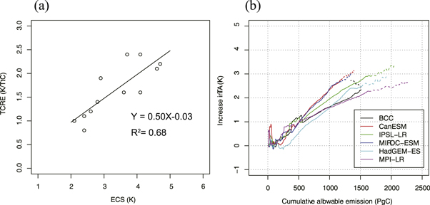
To investigate the consistency of our results with the behaviour of ESMs, we analyzed the output of the CMIP5 models. As shown in figure 4, a clear positive relationship was observed between the ECS and TCRE for the 1 ppa scenario, which is consistent with our results. Figure 4(b) shows the trajectory of six ESMs in the temperature–cumulative-emission plane. Consistent with our results, models with low TCRE at in 2111–2120) have a larger decreasing ratio in TCRE after that. The only model with increasing TCRE after 2111–2120 is the Beijing Climate Center (BCC) model, for which the land carbon storage decreases rapidly after 2111–2120; however, this is actually the only model analyzed that does not calculate land use processes (thus, only for this model, land use emissions are not added to the denominator of TCRE. See figure S1). For all other models, the TCRE decreases after 2111–2120 and the model with the highest TCRE in 2111–2120 was MIROC-ESM (2.3 K/TtC). This model had the lowest rate of decrease until 2291–2300, −1%, while the MPI-LR models had the lowest TCRE (1.4 K/TtC) in 2111–2120 and the largest rate of decrease (−15%) until 2291–2300. A clear positive relationship is observed between the TCRE in 2111–2120 and the ratio of TCRE in 2291–2300 to that in 2111–2120 when the BCC model is removed, although when it is included, the sign of the coefficient of correlation is changed (table S2).
Figure 4. Behaviours of earth system models: (a) relationship between ECS and TCRE for ESMs. ECSs are from Flato et al (2013) and Nohara et al (2015). Values of TCRE are from Gillet et al (2013). (b) Temperature anomaly and cumulative carbon emissions (20 year averages). Data are from historical, RCP4.5 and its extension experiments of CMIP5 (downloaded from the CMIP5 Earth System Grid (http://cmip-pcmdi.llnl.gov/cmip5/) and the Centre for Environmental Data Analysis (http://www.ceda.ac.uk/). The numerator and the denominator of equation (1) are used here. Model drift in temperature is removed by subtracting the linear trend of the first 450 years in the control run. The CO2-induced warming is calculated from ΔT for each model, multiplied by the ratio of CO2-induced and total radiative forcing in the RCP4.5 radiative forcing scenario (http://www.pik-potsdam.de/~mmalte/rcps/). For each model, γ is simply estimated from Arora et al (2013), and the land use emission is common to all models and obtained from the RCP4.5 scenario (Clarke et al 2007, Smith and Wigley 2006, Wise et al 2009). See table S1 for the full names of the models analyzed here.
Download figure:
Standard image High-resolution image
Regarding the limitation of the EMICs, Frolicher and Paynter (2015) argued that the difference in realized warming fraction makes it difficult for the EMICs to represent the behaviours of their ESM in their Phase 2 (i.e., the period between the cessation of CO2 emission and stoppage of OHU). However, in their supplementary table 2, JUMP-LCM (labelled 'MIROC-lite-LCM') is 0.62, which is within the range of GCMs (0.58 ± 0.08). We also confirmed that in our experiment with 512 members, the fraction is 0.71 ± 0.15 at 2110–2120 (for total warming) and 0.59 ± 0.17 at 2065–2074 (same, end of the period with significant increase rate in pCO2). Thus, this point is not significant to the findings of our study.
Nevertheless, we recognise that some features of ESMs cannot be represented by EMICs. For example, Frolicher and Paynter (2015) presented that the GFDL ESM2M model has increasing temperature in Phase 2 for decreasing R–N (radiative forcing–ocean heat uptake). Representing this behaviour is beyond the capability of EMICs (at least, for JUMP-LCM); however, it should also be noted that CSM1 (Frolicher et al 2014), CESM (the successor of CSM1) and MIROC-ESM (Nohara et al 2015) did not show such behaviour and models with such behaviour as GFDL ESM2M do not constitute the majority of the CMIP5 models.
4. Conclusions
We analyzed the output of a prior experiment (Tachiiri et al 2013) with particular focus on the change in the uncertainty of TCRE after atmospheric CO2 concentration is stabilized. We determined that in the dataset, the 90% range of TCRE in 2005 was 0.3–2.4 K/TtC in the unconstrained case and 1.1–1.7 K/TtC when constrained by historical and present-day observational data. The latter figures are consistent with other studies. In our experiment, when the rate of increase in atmospheric CO2 concentration was slowed, TCRE uncertainty began to increase and ultimately, it reached five times that in the early 21st century for the constrained case. A larger TCRE became even larger after stabilization, and a smaller TCRE became even smaller; the key to such change was the land carbon storage. The climate–carbon-cycle feedback for the land ecosystem resulted in negative to small positive carbon uptake after stabilization, constraining the increase in the total allowable emissions after stabilization and subsequent increase of TCRE. In this process, the ECS was important because strong ECS resulted in a large temperature rise before stabilization and substantial climate–carbon-cycle feedback, and large ECS caused a lower level of equilibrium at the start of stabilization and some temperature rise after that. On the other hand, analysis of the CMIP5 models showed some consistency, e.g., a clear positive relationship between the ECS and TCRE for the 1 ppa scenario, and the tendency for models with low TCRE at 2111–20 for the TCRE to decrease between 2111–20 and 2291–2300 (except for the only model not incorporating land use). However, the relationship between the TCRE at 2111–20 and 2291–2300 is less clear than expected from the results for our EMIC. One reason for this could be that all the TCRE of the ESMs were concentrated around the centre of the possible range and no models were near the edge.
If the results showing that larger TCRE result in even greater TCRE following stabilization are correct, then it becomes more difficult to estimate the total amount of carbon that could be emitted for a given climate stabilization target. Thus, careful investigation of the following issues will be important: (1) the contribution of ECS and climate–carbon-cycle feedback for land carbon uptake after stabilization (e.g., constant concentration or zero emissions), and (2) the difference between the behaviours of EMICs and ESMs in such periods. We should also note the expected change after 2300 toward equilibrium, because non-negligible change could occur in that period.
Acknowledgments
This work was supported by the Program for Risk Information on Climate Change, Ministry of Education, Culture, Sports, Science and Technology, Japan. The experiments were performed on the supercomputer system of the Japan Agency for Marine-Earth Science and Technology.