

Abstract
Water temperature controls many biochemical and ecological processes in rivers, and theoretically depends on multiple factors. Here we formulate a model to predict daily averaged river water temperature as a function of air temperature and discharge, with the latter variable being more relevant in some specific cases (e.g., snowmelt-fed rivers, rivers impacted by hydropower production). The model uses a hybrid formulation characterized by a physically based structure associated with a stochastic calibration of the parameters. The interpretation of the parameter values allows for better understanding of river thermal dynamics and the identification of the most relevant factors affecting it. The satisfactory agreement of different versions of the model with measurements in three different rivers (root mean square error smaller than 1oC, at a daily timescale) suggests that the proposed model can represent a useful tool to synthetically describe medium- and long-term behavior, and capture the changes induced by varying external conditions.
Export citation and abstract BibTeX RIS

Content from this work may be used under the terms of the Creative Commons Attribution 3.0 licence. Any further distribution of this work must maintain attribution to the author(s) and the title of the work, journal citation and DOI.
1. Introduction
Water temperature is a crucial factor in almost all ecological and biogeochemical processes in rivers like, for instance, chemical reaction rate, oxygen solubility, primary production, macrobenthos composition, and fish habitat (Caissie 2006, Webb et al 2008). The complexity of river thermal response depends on the temporal and spatial scales, short-term (subdaily) estimates being more challenging since they are affected by a multiplicity of local factors (e.g., cloudiness, vegetation shadowing, topographic heterogeneity), sometimes intermittently. The daily averaged dynamics analyzed in this paper represent a sort of intermediate scale, where the short-term effects are averaged out, albeit the day-by-day variability can still be large. At this temporal scale it is often assumed that air temperature is the main driver (e.g., Caissie et al, 2001, Webb et al, 2003, Sahoo et al 2009), and that it almost completely explains water temperature dynamics if river discharge is also taken into account. Recently, Arismendi et al (2014) wondered whether regression-based statistical models with only air temperature as a predictor could be used to predict stream temperatures in climate projections, an advantageous option because air temperature is a commonly available information. However, they found that these largely used models were not satisfactory even when referring to the more favorable weekly averages, thus opening the way to the implementation of different types of models.
The traditional approach for the prediction of river water temperature is twofold. On the one hand, mechanistic models consider the whole set of physical and thermodynamic processes that affect the thermal dynamics (e.g., Sinokrot and Stefan 1993, Kim and Chapra 1997, Siviglia and Toro 2009), trying to quantify the different terms that concur to define the net heat flux: shortwave solar radiation, longwave radiation emitted by the water body and the atmosphere, latent and sensible fluxes, effect of inflows and outflows, etc. On the other hand, linear and nonlinear regressions primarily dependent on air temperature (e.g., Mohseni and Stefan 1999, Morrill et al, 2005), or different types of stochastic models (Caissie 2006, Benyahya et al 2007), have been introduced to mimic the behavior of river water temperature interpreted as a purely statistical variable, thus renouncing the physical description of the thermal dynamics. The two approaches have complementary strengths and drawbacks. Physical models require a large number of input data (including stream geometry, vegetation cover, land use, and meteorological conditions), and evaluate the heat flux components through empirical relationships, which are affected by uncertainties and require quantities difficult to measure or estimate, especially for non-radiative fluxes. Purely statistical models are not able to provide a physical justification to their structure, so the extrapolation of the results to unobserved conditions is always questionable (e.g., Benyahya et al 2007). This is particularly the case of regression models, which are intrinsically valid only in the range of measured values.
In this paper we propose an intermediate approach. Starting from the governing physical relationships, we derive a new model (termed air2stream) characterized by limited computational complexity, comparable to that of statistical models. The final structure is that of a single ordinary differential equation linearly dependent on air and water temperature, and discharge. Differently from the mechanistic models, the extremely simple formulation allows for calibration of the model parameters by means of a Monte Carlo-like method. Thus, the model can be seen as a hybrid tool that is physically based, but takes advantage from the data to inform its structure, in a way that resembles neural networks (e.g., Sahoo et al 2009). We successfully tested a similar approach to predict lake surface temperature based on air temperature alone (Piccolroaz et al 2013) obtaining satisfactory results in a wide range of different lake morphologies (Toffolon et al 2014) and conditions (Piccolroaz et al 2015). In this paper we extend this approach to a different context where other factors (like discharge) may become influential. We also derive a set of simpler versions of the model by neglecting some elements and introducing the assumption of instantaneous adaptation to the external conditions. The performance of the different versions are tested against the logistic function model (i.e., one of the most popular nonlinear regression models) considering three significant case studies in Switzerland characterized by different hydraulic regimes: natural, regulated and snow-fed rivers.
2. Materials and methods
2.1. Case studies
In order to test performances of the model, we have selected three rivers in Switzerland characterized by different hydrological conditions. The three cases are briefly described below and in table 1 (for further details please refer to the supplementary material). For a more extensive description of the Swiss database see, e.g., Schaefli et al (2015).
- 1.The river Mentue flows at low altitude on the Swiss plateau through a sparsely inhabited area with predominant agricultural land use, unaffected by strong anthropic thermal alterations. This case is representative of the typical conditions of a small 'natural low-land' river.
- 2.The station of the river Rhône at Sion lies at the bottom of a populated alpine valley. Starting from the beginning of the 20th century its hydrological regime has been altered by the construction of a large high-head hydropower storage system, and the river is now affected by strong hydro- and thermo-peaking (Meile et al, 2011). This case is considered as representative of a strongly 'regulated' river.
- 3.The river Dischmabach is located at high altitude in a steep glacial valley that is uninhabited and used for mountain pastures, with a significant influence of snow melting. This case is taken as a representative example of a 'snowmelt-fed' river.
Table 1. Characteristics of river and meteorological stations.
| Case | 1 | 2 | 3 |
| River name | Mentue | Rhône | Dischmabach |
| Classification | natural low-land | regulated | snow-fed |
| River station name | Yvonand | Sion | Davos |
| (La Mauguettaz) | (Kriegsmatte) | ||
| River station code (Tw, Q) | 2369 | 2011 | 2327 |
| River station elevation [m a.s.l.] | 449 | 484 | 1668 |
| Catchment average elevation [m a.s.l.] | 679 | 2310 | 2372 |
| Catchment area [km2] | 105 | 3373 | 43.3 |
| Calibration period | 2002–2009 | 1984–2003 | 2003–2009 |
| Validation period | 2010–2012 | 2004–2013 | 2010–2012 |
| Meteo station name | Mathod | Sion | Davos |
| Meteo station code (Ta) | MAH | SIO | DAV |
| Meteo station elevation [m a.s.l.] | 437 | 482 | 1594 |
| Distance from river station [km] | 12.7 | 2.14 | 4.90 |
2.2. Formulation of the model
The model is based on a lumped heat budget that considers an unknown volume V of the river reach, its tributaries (implicitly considering both surface and subsurface water fluxes), and the heat exchange with the atmosphere, as depicted in figure 1. The variation of water temperature Tw in this volume is governed by the equation
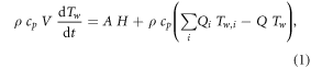
where t is time (hereafter expressed in days), ρ is water density, cp its specific heat capacity at constant pressure, A is the surface area of the river reach, H is the net heat flux at the river-atmosphere interface, Q is the discharge at the downstream section, Qi and Twi are discharge and temperature of the i-th contributing water flux (tributaries and, possibly, groundwater), and V is the total volume that reacts to the heat fluxes. We notice that V is not necessarily limited to the surface water body, possibly including also the hyporheic region, so that the explicit inclusion of heat fluxes at the stream-river bed interface is not necessary.

Figure 1. Schematic representation of a river reach with relevant inflows and heat fluxes.
Download figure:
Standard image High-resolution imageThe first term on the right hand side of equation (1) contains the net heat flux H, which is primarily a function of short- and long-wave radiation, and latent and sensible heat fluxes. Following Caissie (2006), we assume that air temperature, Ta, can be used as a proxy for all these processes. The overall effect is included in the model in a linear form by using a Taylor series expansion (similarly to as in Piccolroaz et al (2013), see details in the supplementary material), such that
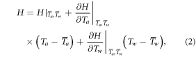
where  and
and  are the long-term averaged values (hereafter indicated by an overbar) of air and water temperatures, respectively. This relation can also be rewritten as

where h0, ha and hw are parameters that can be directly derived from equation (2).
The second term on the right hand side of equation (1) represents the difference between the heat flux leaving the control volume,  and the sum of all the entering heat fluxes. These are almost impossible to determine precisely, and are inherently case-specific. Noting that
  we introduce a fictitious mean inflow temperature
  Such a reference temperature is likely to change in the different seasons, so we express it as a first approximation in the form of sinusoidal annual variation
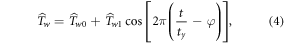
where the reference value  the amplitude of the variation
  and the phase
 ![$\varphi \in [0,1]$](https://content.cld.iop.org/journals/1748-9326/10/11/114011/revision1/erl521169ieqn8.gif) are left unspecified, with ty being the duration of a year expressed in the same units as t.
are left unspecified, with ty being the duration of a year expressed in the same units as t.
Thus, we can rewrite equation (1) as
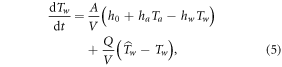
which contains two characteristic quantities. The inverse of the first ratio, V/A, is related to the flow depth D (and hence depends on the discharge), but does not coincide with it. In fact, a portion of the saturated sediments should be included, especially for shallow flows with high transparency where the incoming shortwave radiation can directly warm the river bed (Evans et al, 1998, Caissie 2006). The second ratio in the equation, Q/V, represents the inverse of the residence time in the river reach, and varies with the discharge as well. In order to allow for an explicit dependence of these two ratios on easily measurable quantities, we introduce the dimensionless reference volume, δ, and we assume a simple power law as a function of the discharge:

where  is the dimensionless discharge and m is related with the exponent of the rating curve (e.g.,
  according to the Manning's normal flow relationship in a wide rectangular channel). Introducing these relations into equation (5), we obtain the final form of the air2stream model
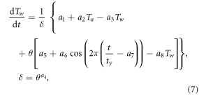
where the eight parameters a1–a8 of the model (7) directly follow from equations (3), (4) and (6). It is important to stress that the values of these parameters are estimated through calibration, so that all the geometrical characteristics of the river reach (length, volume, area, etc) are not required to be explicitly specified, nor the role of specific heat inputs (e.g., internal friction). This feature of the model also implies that local effects, such as that of shading, are expected to be automatically captured by the calibration of the parameters. However, we note that there are cases where air temperature and discharge alone may not be sufficient for an accurate estimate of the net heat flux. A possible example is given by rivers affected by intermittent industrial point releases generally characterized by modest water fluxes at relatively high temperature, whose effect on stream thermal dynamics may be difficult to reproduce especially when these releases are irregular.
Equation (7) resembles the model air2water developed by Piccolroaz et al (2013) for lakes and reservoirs. However, two main differences exist: (i) rivers are typically not stratified, so δ is not a function of Tw, but rather of Q; and (ii) the effect of the contributing water fluxes, both natural and regulated (e.g., affected by hydropower release), is included as it can be substantial for some types of rivers and under specific circumstances. With particular reference to the second point, here we propose a few alternative versions of the 8-parameter formulation (7).
2.3. Other versions of the model
The first variation comes from disregarding the second term on the right hand side of equation (1). The resulting 4-parameter model reads

and corresponds to assuming that the mean temperature of the contributing water fluxes is approximately equal to that of the river (i.e.,  ). Another case in which the model (8) is valid is when these fluxes are absent or their effect is not relevant, so that
  is close to the temperature of the river at the upstream end of the considered reach. In general, this model can be successfully applied if the longitudinal gradient of temperature is small.
We will see in the following analysis that the effect of δ is minor in the three examined cases, which implies that the thermal response of the river does not strongly depend on the flow depth at a daily timescale. Therefore, we identify two new versions of the model by setting  (i.e.,
  ): a 7-parameter model derived from (7), and a 3-parameter model derived from (8). The latter model is the simplest that can be used to simulate river temperature variations.
A further version of the model can be obtained by simplifying the 7-parameter version imposing also  i.e. assuming that the effect of the discharge can be approximately retained using only a constant value. In this way, by combining the constant terms and those proportional to Tw, we obtain a 5-parameter version
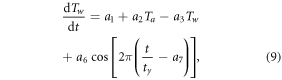
where the interpretation of the parameters a1, a3 and a6 changes from that of the initial model. The summary of the five versions of the air2stream model is reported in table 2 (the source code is available at https://github.com/marcotoffolon/air2stream).
Table 2. Versions of the model and performances for the three case studies.
| Version | Parametersa | RMSE Tw [°C] (NSE [−]) | ||||||||||||||
| of the | a1 | a2 | a3 | a4 | a5 | a6 | a7 | a8 | δ | θ | Case 1 | Case 2 | Case 3 | |||
| model | calb | valc | cal | val | cal | val | ||||||||||
| 8-par | x | x | x | x | x | x | x | x |

|
θ | 0.62 (0.99) | 0.76 (0.98) | 0.58 (0.92) | 0.75 (0.89) | 0.61 (0.96) | 0.62 (0.95) |
| 7-par | x | x | x | — | x | x | x | x | 1 | θ | 0.62 (0.99) | 0.78 (0.98) | 0.61 (0.92) | 0.77 (0.89) | 0.64 (0.95) | 0.65 (0.95) |
| 5-par | x | x | x | — | — | x | x | — | 1 | — | 0.65 (0.99) | 0.78 (0.98) | 0.88 (0.83) | 1.05 (0.79) | 0.70 (0.94) | 0.70 (0.94) |
| 4-par | x | x | x | x | — | — | — | — |

|
— | 0.77 (0.98) | 0.92 (0.98) | 0.90 (0.81) | 1.04 (0.79) | 0.88 (0.91) | 0.87 (0.91) |
| 3-par | x | x | x | — | — | — | — | — | 1 | — | 0.78 (0.98) | 0.91 (0.98) | 0.91 (0.81) | 1.05 (0.79) | 0.89 (0.90) | 0.88 (0.91) |
 from 8-par (6 parameters) from 8-par (6 parameters) |
— | θ | 0.71 (0.99) | 0.83 (0.98) | 0.59 (0.92) | 0.75 (0.89) | 0.64 (0.95) | 0.66 (0.95) | ||||||||
 from 5-par (4 parameters) from 5-par (4 parameters) |
— | — | 0.72 (0.98) | 0.83 (0.98) | 0.87 (0.83) | 1.05 (0.79) | 0.76 (0.93) | 0.78 (0.93) | ||||||||
 from 4-par (2 parameters) from 4-par (2 parameters) |
— | — | 0.96 (0.97) | 1.07 (0.97) | 0.91 (0.82) | 1.05 (0.79) | 0.94 (0.89) | 0.94 (0.89) | ||||||||
| Logistic regression (4 parameters) | — | — | 0.98 (0.97) | 1.10 (0.97) | 0.71 (0.89) | 0.86 (0.86) | 0.89 (0.90) | 0.89 (0.90) | ||||||||
a'x' denotes parameters that are calibrated, '-' parameters that are not included in the version of the model. bCalibration. cValidation.
2.4. Calibration of the model
The successful application of the model relies on a careful calibration. The best set of parameters is identified by defining a physically reasonable range of the parameter values and solving an optimization problem. The aim is to minimize the error between simulated and measured water temperatures, defined through the introduction of a suitable metric (objective function). The input data are a continuous series of daily averaged air temperature and river discharge (the latter only for some versions, see table 2). The output of the model is the series of daily averaged water temperature, which is compared with measured values. In the most favourable case, observed water temperature is a series of continuous daily values, but the model can be calibrated also with a reduced number of data or aggregated values (e.g., weekly or monthly averages, see Toffolon et al (2014) for lakes). Air and water temperature series should be long enough to capture interannual variability, thus in general should extend for several years. As a general rule, we used 2/3 of the available series for calibration and 1/3 for validation of the model.
The objective function used for model calibration is the root mean square error (RMSE) between simulated and observed Tw. Moreover, we calculated the Nash-Sutcliffe Efficiency (NSE) index that normalizes the variance of the errors with the variance of the measurements (Moriasi et al, 2007). We recall that NSE equal to 1 corresponds to perfect agreement, while negative values indicate that the mean would have been a better predictor than the tested model.
The identification of the best set of parameters for each river is performed through a Monte Carlo-based optimization procedure in which a large number of parameter sets is sampled and evaluated in terms of RMSE. Here we use the particle swarm optimization (PSO) algorithm, a population-based stochastic optimization technique firstly proposed by Kennedy and Eberhart (1995) (see supplementary materials for further details) with a population of 1000 particles and for 1000 iterations. For each run, equation (7), or any other version of the model, is numerically integrated using the Runge–Kutta 4th order method with a time step of one day. Computed water temperatures below 0oC have been limited to that value.
3. Results and discussion
3.1. Performances
The five versions of the model were applied to the three case studies (table 1), showing a general good agreement between model results and measured water temperature. Table 2 reports the values of RMSE, which are always smaller than 1oC in calibration (i.e., first 2/3 of the series), with only minor increases for some cases in validation. The values of NSE are also reported, which are always larger than 0.8 and in some cases very close to 1, thus suggesting that the model performs well also in relative terms.
In order to visually appreciate seasonal fluctuations in temperature and discharge of the three case studies, we calculated the reference year (daily means) of all variables (measured air and water temperature, discharge, and modeled water temperature) by averaging across all years the values for each day of the year. Figure 2 shows the performances of the 8-parameter version (the results of the other versions and the values of the parameters are reported in the supplementary material) and demonstrates that the model effectively follows the measured annual oscillation. We note that the phase is not necessarily coincident with that of Ta because of the contribution of Q and of the additional sinusoidal term, possibly characterized by a different phase.
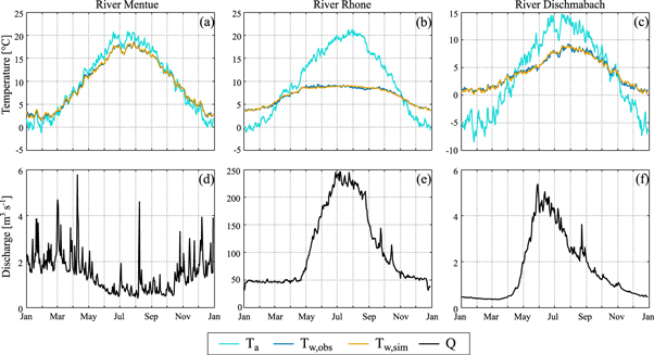
Figure 2. Reference year of the variables for the three case studies (columns): (a)–(c) measured air temperature (Ta), and observed ( ) and simulated (
 8-parameter model) water temperature; (d)–(f) measured discharge (Q).
Download figure:
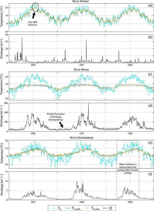
Standard image High-resolution imageInterannual variability of river water temperature is examined in figure 3 during a period of three years. For all rivers the model is able to reproduce the sequence of cold and warm years, as for example the particularly warm 2006 summer and 2006/2007 winter in case 1, the warm 1987/1988 winter in case 2, and the cold 2008 spring in case 3 associated with the occurrence of larger discharge values.
Figure 3. Interannual variability of air and water temperature and discharge for the three case studies: case 1 (a)–(b), case 2 (c)–(d), and case 3 (e)–(f). The model is applied in the 8-parameter version.
Download figure:
Standard image High-resolution image
The three examined rivers behave in a markedly different way. The response of water temperature to changes in air temperature is almost linear for the low-altitude river (case 1), thus producing large differences between annual maximum and minimum water temperature. Indeed, case 1 is characterized by a relatively low discharge, which typically corresponds to a shallow depth and hence a low thermal inertia (but larger lowland rivers may behave differently). Conversely, although at the same altitude, case 2 presents a much more limited increase of water temperature, especially in summer. This is attributable to the release of cold water during hydropower production, which has been shown to affect the thermal behavior of the rivers at different temporal scales (Zolezzi et al, 2011). Since thermal alterations travel for long distances (Toffolon et al, 2010), the impact can be felt along the whole river in alpine contexts, especially if there are not other significant tributaries. The resulting effect is a marked flattening of the natural seasonal pattern (Meier and Wüest 2004). Finally, water temperature in case 3 is generally low during the whole year because of the high altitude and the contribution of snow melting waters (Lisi et al, 2015). The influence of an upstream snowfield is clearly distinguishable in the abrupt variations of the discharge due to snow melting starting in spring and slowly decreasing during summer and autumn, with almost no flow in winter. The effect of the cold melting water is similar to that of hydropower releases: a much lower response of Tw to Ta during the warm season. We also note that a large contribution of cold groundwater inputs can produce similar effects (Tague et al, 2007).
For the selected cases, and over the specific study periods, the 8-parameter model always performs better than the other versions (table 2), but the improvement is different in the three types of rivers. In particular, the effect of discharge cannot be neglected in case 2 (strong influence of hydropower generation) and case 3 (significant contribution of snow melt) because the water flowing at the river station originates from a number of colder contributions. As a result, the model depending on air temperature only is not suitable to reproduce the proper dynamics, although the 5-parameter version yields a substantial improvement without considering Q explicitly. This is particularly true for case 3, for which the phase shift induced by the additional sinusoidal term (representing the mean inflow temperature) is able to postpone the warming of the river water with respect to that of the air in spring, mimicking the effect of cold contributions due to snow melting water. Conversely, the effect of discharge is not so relevant in case 1, and the 3-parameter version already produces satisfactory results (table 2). In this case, the river does not receive large tributaries, so its temperature is approximately spatially uniform along large distances (i.e.,  ). Anyway, a significant improvement is given by the 5-parameter model, which compensates the small phase lag that is however present between air and water temperature, and by the 7- and 8-parameter models, despite Q is less variable during the year than in the other two rivers.
3.2. Adaptation time scale and equilibrium temperature
Interestingly, the performances of the 7-parameter and 3-parameter versions are comparable to those of the 8-parameter and 4-parameter versions, respectively, for the three examined rivers. This suggests that the role of δ, which represents the variation of the thermal inertia of the river as a function of Q, is minor. This result seems to contradict the common intuition that smaller flow depths (due to smaller Q) would result in a warmer river water temperature in summer, and, conversely, in a colder river water temperature in winter. Actually, δ influences the reaction time to external forcing, but not the value at equilibrium. This can be easily shown by considering the structure of the model, as it is discussed in the supplementary material where analytical solutions are derived in idealized cases. There, we show that  (with
(with  for the 8-parameter model) controls the time scale for the adaptation of Tw to the external forcing. Referring for simplicity to the 5-parameter model (9), which does not include θ (hence
  ), and assuming
  the time scale is 0.94, 0.55 and 0.36 days for cases 1, 2 and 3, respectively. This means that water temperature adapts to the external forcing in a period that is comparable with the averaging window (1 day) assumed in this analysis. Such a consideration can be supported by rewriting equation (7) as
from which it clearly appears that when A3 is large compared to the temperature variations (multiplied by δ, which however is  on average) the left hand side vanishes. A more precise condition has been derived in the supplementary material by also taking the time derivative into account by means of a perturbation method: the ratio
  (where A2 represent the amplitude of an approximately equivalent sinusoidal forcing) has to be lower than a threshold, confirming the strong inverse dependence on A3. When such a condition holds, the thermal response becomes substantially independent of δ and an instantaneous equilibrium water temperature
  can be adopted as an approximation (Caissie et al, 2005).
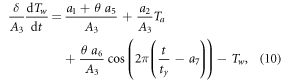
Neglecting the time derivative in equation (10) and rearranging the parameters by dividing everything by a3, the 8-parameter and 7-parameter versions reduce to
where  ,
,  ,
,  ,
,  ,
,  , and
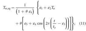
, and  The approximation (11) explicitly illustrates how the effect of the discharge is felt only through θ, suggesting that, besides the exchanges with the atmosphere, it is the contribution of the inflows (with a temperature that may be different from that of the receiving river) that relevantly affects water temperature. Similarly to equation (11), the 5-parameter version reduces to
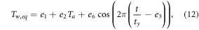
and the 4-parameter and 3-parameter versions to

These equilibrium relationships are characterized by a number of parameters that is smaller than the original model because a3 is used to rescale the other parameters. Thus, equation (11) is characterized by only 6 parameters to calibrate. The other relationships (12) and (13) have only 4 and 2 free parameters, respectively, the latter representing the equivalent of a linear regression with a lower bound at 0 oC. The performances of the equilibrium relationships are compared with the complete models in table 2. In the same table, we also report the RMSE and NSE of the most widely used nonlinear regression model, based on the logistic function (e.g., Arismendi et al, 2014), whose formulation is explicitly presented in the supplementary material and contains 4 parameters to calibrate. The 8- and 7-parameter versions of air2stream outperform the logistic regression for all rivers, both in the differential form and under the equilibrium assumption. The other versions have higher performances, as well, with the only exception of case 2. In the regulated river, in fact, the S-shape of the logistic function is able to capture the flattening of water temperature in summer, but does not account for the actual physics governing the thermal process. The information about Q is indeed essential, that is the reason why the simplest versions of the model are less adequate. In conclusion, our model performs better than the common statistical models and moreover includes the most relevant physical factors. A direct comparison is not possible with fully mechanistic models, which would require much more information. Finally, we note that, differently from the linear and nonlinear regression models that can reproduce only a biunivocal dependence of Tw as a function of Ta, the solutions (11) and (12) allow for a more realistic hysteretic pattern Tw-Ta, despite the complexity of the formulation is equivalent.
4. Conclusions
The proposed model, which is termed air2stream in analogy to the model air2water developed for lentic waters like lakes (Piccolroaz et al, 2013), is a powerful tool that can help in investigating the thermal dynamics of various types of rivers in a simple and effective way. The model is dependent on daily values of air temperature and flow discharge only, two variables that are measured in many rivers. This extremely basic input data set makes the model a flexible instrument that is prone to many practical applications.
The model is formulated in different versions, which represent reduced formulations of the fundamental model with 8 parameters. The analysis of the results of the five versions of the model highlights the relative importance of the different factors (particularly the discharge) that drive the thermal response in rivers. Furthermore, three equilibrium solutions are derived from the complete differential model, which are valid when the adaptation time scale is short with respect to the averaging window of the measurements.
Model calibration, together with the simple yet physically-based structure of the model, represents the crucial aspect of the approach, whereby data inform the model without the need to rely on empirical formulations and on a large mass of geometrical and hydraulic data. The possibility of grasping the very basic physics behind the thermal process without specifying unnecessary details suggests that this approach may be more effective than standard mechanistic models, which would require additional inputs that are usually unavailable. Indeed, the performances of our model are extremely good (average RMSE in the three cases is 0.60 oC in calibration and 0.72 oC in validation, at a daily scale) without the need to consider local shading, cloud cover, atmospheric influences, or the temporal variability of the various forcings. Moreover, the formulation does not require to understand the location of the upstream boundary condition or where (and how) significant inflows come into the model area, whether as surface water or groundwater. Reconstructing this information would need an extremely detailed analysis of the watershed and the implementation of a reliable hydrological model, a task that is generally not within the reach of standard applications.
At the same time, being based on physical grounds, air2stream overcomes the limitations of typical regression models, which do not allow for future extrapolation as their validity is limited by the range of past observations (e.g., Mohseni and Stefan 1999). An obvious application in this sense is the use of the model in long-term climate studies, especially in its simpler formulations. In fact, up to the 5-parameter version the model would not need to reconstruct the expected river discharges, but only the scenarios of air temperature, which are the common (and likely the most reliable) output of global climate studies. We are aware that the analysis of three cases, although characterized by markedly different hydrological regimes, is not sufficient to provide a definitive evidence of the broad applicability of the model. However, we can anticipate that the preliminary results from an ongoing comparative study using a larger data set of rivers are very promising. A deeper analysis of the robustness of the model and its potential for long-term studies is also currently being performed. This analysis is aimed at understanding whether air temperature is a sufficiently good proxy for water temperature, also in those cases where thermal gradients between the main stream, tributaries and groundwater fluxes are expected to be altered significantly as a consequence, for instance, of changes in snowfall patterns.
In the end, we were able to address the main question raised by Arismendi et al (2014) by showing that air temperature can be satisfactorily used as the sole input if the model is suitably designed (as in the 5-parameter version), and that the role of discharge becomes influential when snowmelt input is dominant, and essential only in the case of heavily regulated rivers.
Acknowledgments
Water temperature and discharge data were kindly provided by the Swiss Federal Office of the Environment (FOEN), and meteorological data by the Swiss Meteorological Institute (MeteoSchweiz). We are grateful to Elisa Calamita for the precious contribution in the analysis of the data, to Annunziato Siviglia (ETHZ, Switzerland), Aurélien Gallice (EPFL, Switzerland) and Bruno Majone for discussing various analyses used in preparation of the manuscript, and to Martin Schmid, Guido Zolezzi and Bettina Schaefli for valuable comments on a first draft. The source code of the air2stream model is freely available at https://github.com/marcotoffolon/air2stream, together with the data from the three case studies.