


Abstract
Accurate and traceable measurements of transmittance haze are required for quality control in various different industries, such as optoelectronics, automobiles, and agriculture. Transmittance haze is defined as the fraction of light transmitted through a material that deviates from the incident beam by more than 2.5∘. Various documentary standards specify the use of an integrating sphere with a prescribed geometry for the measurement of transmittance haze. This paper uses goniometric measurements of the bidirectional transmittance distribution function (BTDF) to calculate transmittance haze according to the definition and demonstrates that the sphere-based realisation of transmittance haze specified in the documentary standards does not agree with the definition, with the difference being up to 20% for some samples. The BTDF measurements are also used to simulate the integrating sphere haze, allowing the sensitivity of the sphere haze to errors in the integrating sphere geometry to be calculated.
Export citation and abstract BibTeX RIS
1. Introduction
The degree to which light scatters as it passes through materials is of interest for many applications in a wide range of industries, including optoelectronics, automobiles, and agriculture. For some applications, we want to be able to control and eliminate scattering, such as for telescope optics, car windscreens, and window tinting. For other applications, we want to increase light scattering, for example for privacy glass and agricultural fabrics. There are also cases where we want to be able to track the scattering as a function of composition, processing, or damage, such as for recycled plastics and screen protectors for hand-held electronic devices or electrical appliances.
One way of quantifying this scattering is to measure the transmittance haze of a material. According to the CIE International Lighting Vocabulary [1], transmittance haze is defined as the fraction of transmitted light that is scattered by more than a specified angle, referred to in this paper as the cut-off angle, from the direction of the incident beam. The International Lighting Vocabulary also specifies the effect of transmittance haze on a material being a 'reduction in contrast of objects viewed through it'. This suggests that the scattering angle must be high—if the scattering was only at small angles, we would expect a loss in resolution, rather than a loss in contrast.
There are several different documentary standards describing an instrument for the measurement of transmittance haze [2–5]. The various standards all agree on the definition of haze as the percentage of transmitted light that deviates from the incident beam by more than 2.5∘. They also agree on the realisation of haze using an integrating sphere with a prescribed geometry, which is illustrated in figure 1. The integrating sphere should have at least two ports: an entrance port and an exit port directly opposite the entrance port. The exit port should subtend 8∘ from the centre of the entrance port. A collimated beam should be used for the measurements, and there should be an annulus around the collimated beam at the exit port that subtends 1.3∘ from the centre of the entrance port.

Figure 1. Diagram showing the simplified integrating sphere geometry specified by the documentary standards for measurements of transmittance haze with no sample (left) and with a scattering sample mounted on the entrance port of the sphere (right). The exit port subtends 8∘ from the centre of the entrance port, a collimated beam is used, and there is an annulus around the collimated beam at the exit port that subtends 1.3∘ from the centre of the entrance port.
Download figure:
Standard image High-resolution imageWhen a transmitting sample is placed on the entrance port, the regularly transmitted light, and light scattered to low angles, is lost through the exit port, while the light scattered to higher angles is captured inside the sphere and is measured from a detector port (not shown in figure 1) to determine the diffuse transmittance of the sample. If the exit port is plugged with the same material as the internal surface of the sphere, all the light transmitted by the sample is captured in the sphere, and the total transmittance can be measured. The realisation haze can then be calculated using the formulae specified in the documentary standards.
While the standards all agree on the definition of transmittance haze and the geometry of the integrating sphere used for the measurements, the standards differ in the specified sphere configurations for the measurements. In the ASTM D1003 standard [2], the components on the integrating sphere are removed and replaced for the different measurements, which causes the sphere throughput to vary. This causes the measured haze to vary depending on the sphere multiplier, with differences in the haze value of up to 15% obtained using two different spheres, both complying with the standard [6, 7]. On the other hand, the ISO 14782 [3] and BS 2782-5 [5] standards, as well as the center for measurement standards (CMS) method [8] (which has been shown to give the same haze values as the ISO 14782 standard [9]) specify the use of a compensation port to keep the sphere throughput consistent. This means that the same haze value is obtained when measuring with different spheres, but this value is different to the value obtained following the ASTM standard [9].
Aside from the differences in the haze values measured according to different standards, it is also worth looking at how well the sphere measurement approximates a realisation of the definition of haze given in the standards. The definition requires beams scattered by more than 2.5∘ to be separated from those scattered by less than that. Achieving this would require an infinitesimal beam, so the specified integrating sphere geometry makes an approximation that induces an error depending on the sample and its bidirectional transmittance distribution function (BTDF). Using a goniospectrophotometer, the BTDF can be measured over the hemisphere. Then, by integrating the appropriate parts of the BTDF, the definitional haze can be calculated according to the definition given in the documentary standards. Sphere-based approximations of transmittance haze are used in the documentary standards because they are a much faster and easier way of measuring haze than using a goniospectrophotometer to make measurements of BTDF over the hemisphere, which then need to be integrated.
In this paper, measurements of BTDF made using a goniospectrophotomter are used to measure the definitional haze for three samples according to the definition given in the documentary standards. These haze values are compared to the realisation haze values measured using an integrating sphere according to the documentary standards. Firstly, the BTDF measurements of the samples are presented. Then, the method of integrating BTDF measurements to estimate the sphere-based value is validated by integrating the BTDF over the hemisphere to calculate the total transmittance. This confirms that the same scales are realised using the integrating sphere and goniospectrophotometer so that any differences observed in the haze measurements are meaningful. Then, the definitional and realisation haze values are compared. Finally, the BTDF measurements are used to simulate the transmittance haze measured using an integrating sphere. This enables the estimation of the sensitivity of the sphere haze to parameters that are difficult to physically vary in an instrument, such as the exit port diameter and the incident beam diameter.
2. BTDF and total transmittance
The BTDF,  , of a sample describes the transmittance of light in a given direction [10]. It is a function of the polar and azimuthal angles of incidence,
  , and detection,
  , and the wavelength of the incident flux, λ [11], and can be measured using a four-axis goniometric system. In the MSL and CNAM systems, which both have a collimated incident beam that is smaller than the sample and the detector aperture, the BTDF can be expressed as
where  and
and  are the incident and detected fluxes, respectively, and
  is the solid angle of detection, which depends on both the distance between the sample and the detector, L, and the surface area of the detector, A. The solid angle is given by
The BTDF is also dependent on the polarisation of the incident flux and is typically measured using unpolarised incident illumination (typically achieved by averaging measurements made with each of s- and p-polarised light). Figure 2 shows the geometry of the incidence and detection angles in the BTDF definition.

Figure 2. Schematic diagram showing the angles  in the BTDF definition. Note that, here, the transmitted beam is passing through the sample.
Download figure:
Standard image High-resolution image2.1. Total transmittance
The total transmittance,  , is defined as the fraction of the incident radiant flux that is transmitted through the sample [1]. The total transmittance can be calculated by integrating the BTDF measured with normal incidence over the whole hemisphere—from
  to
to  and
and  to
to  [12]:
[12]:
where  is the BTDF at θd averaged over φd and the integral is evaluated analytically from a cubic spline fitted to the measured values.
3. Samples and BTDF measurements
The work described in this paper was carried out using three different types of sample: two cellulose nanofibril samples, 5P-2 and 5P-3, with a high total transmittance and a narrow BTDF peak at  , produced at RISE; a holographic diffusing sample, H5, with a high total transmittance and a wider BTDF peak than the cellulose nanofibril samples; and a quasi-Lambertian sintered halon sample, H2, with a much lower total transmittance and a high haze value, produced at MSL. All three sample types are isotropic.
BTDF measurements of these samples were made using the goniospectrophotometers at MSL [12] and at CNAM [13]. Figure 3 shows the shapes of the BTDFs for the three sample types over the hemisphere, measured at MSL using 550 nm light with normal incidence, averaging measurements made using s- and p-polarised incident light, and averaged over φd. 5P-2 has a very sharp and narrow peak in the centre, with the BTDF dropping quickly outside the central peak, then more slowly over the rest of the hemisphere. H5 has a wider peak in the centre than 5P-2, but then the BTDF drops off much more outside the peak, with the signal getting quite low and noisy at around  . H2 has a very flat BTDF across the hemisphere.

Figure 3. BTDFs of the three samples used for this work measured with 550 nm light with normal incidence and averaged over φd, plotted on a log-linear scale. The relative standard uncertainties in these values vary between 0.16% and 10%, with the uncertainty increasing at larger θd angles for the H5 and 5P-2 samples.
Download figure:
Standard image High-resolution imageMeasurements of the cellulose nanofibril sample, 5P-3, and the holographic diffusing sample, H5, were also made using the ConDOR facility at CNAM, providing very high resolution measurements over the central peaks. Figure 4 shows the BTDF of the 5P-3 sample and figure 5 shows the BTDF of the H5 sample each measured using Illuminant A with a V(λ) filter. Each pixel in these plots corresponds to a BTDF measurement at one angular position ( ), where θd increases along the radius and φd is plotted as the polar angle. In figure 4, the sharp and narrow BTDF peak of the cellulose nanofibrils sample is clearly resolved, with the BTDF dropping quickly outside the peak.
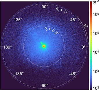
Figure 4. BTDF of the cellulose nanofibrils sample measured using ConDOR [13] under Illuminant A with a V(λ) filter between  and
and  .
.
Download figure:
Standard image High-resolution image
Figure 5. BTDF of the holographic diffusing sample, H5, measured using ConDOR [13] under Illuminant A with a V(λ) filter between  and
and  .
.
Download figure:
Standard image High-resolution imagePhotographs of the three samples are shown in figure 6, with each sample being held at distances 0 mm, 50 mm, and 120 mm from the background sheet of paper. These images demonstrate the visual effects of each type of sample. For the H2 sample, the total transmittance is low, so the text behind the sample cannot be seen in any of the images. The 5P-2 sample has a very high BTDF peak at  , so a lot of light is regularly transmitted and we can read the text behind the sample at all three distances, but there is a loss of contrast due to wide-angle scattering. On the other hand, the H5 sample has a wide BTDF peak, with light scattered out to
  . When the text is immediately behind the sample, most of the light goes straight through and we can still read the text. However, when the sample is held further from the text, the light passing through the sample is scattered by a larger angle and the text has a further loss of distinctness so that we can no longer read it.
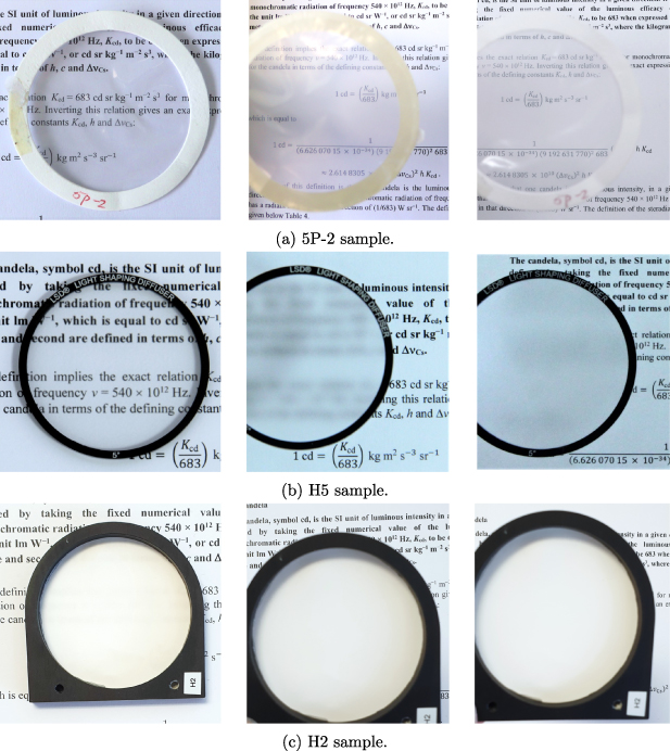
Figure 6. Photographs of the 5P-2, H5, and H2 samples taken with the sample held at distances 0 mm (left), 50 mm (centre), and 120 mm (right) from the background sheet of paper.
Download figure:
Standard image High-resolution image4. Calculating haze from BTDF
Despite being the standard method of measuring haze, integrating spheres can only give an approximation of the transmittance haze of a sample—the realisation haze. Since the beam is usually large relative to the port size, which often has a large diameter, the percentage of light deviating by more than 2.5∘ cannot be accurately measured using an integrating sphere (see below). Instead, the definitional haze can be realised by integrating the measurements of BTDF made using a goniospectrophotometer.
4.1. Integration of BTDF
Many transmitting samples have high, narrow peaks in their BTDFs at small detection angles. Calculating the total transmittance for this type of sample using equation (3) will underestimate the total transmittance, sometimes by up to 50%. This is because the  weighting gives the BTDF measured at
  no weighting in the integral as it assumes that the BTDF measurements were made using a point source and an infinitesimal detector with very small steps between measurements. Since the measurements must be made over a finite solid angle, which is limited by the instrument function, this assumption clearly does not hold in practice. For many transmitting samples, the BTDF measured at
  can have a significant contribution to the total transmittance. In this case, the integral should be calculated by summing areas and signals.
Instead of weighting each measurement using  , the measurements can be weighted based on the relative area of the spherical annulus sampled by the detector for each measurement. Assuming that the sample is isotropic, the total amount of light scattered by a given polar angle θd can be calculated by dividing the measured signal at this angle by the area of the detector aperture and then multiplying by the area of the fraction of the hemisphere (i.e. the spherical annulus) corresponding to this angle. By summing up all the transmitted light in this way, the total transmittance can be calculated as
where  is the flux ratio,
  , measured at the polar angle θi
,
, measured at the polar angle θi
,  is the area of the detector aperture, and
  is the corresponding area of the spherical annulus centred on θi
, where L is the distance between the sample and detector. For the measurement at
is the corresponding area of the spherical annulus centred on θi
, where L is the distance between the sample and detector. For the measurement at  (i = 1), the area begins at θi
and when i = N, the area ends at θN
.
(i = 1), the area begins at θi
and when i = N, the area ends at θN
.
This is illustrated in figure 7. Suppose that measurements of the scattered signal were made at polar angles corresponding to the solid lines in the diagram. Then, the surface area of the hemisphere corresponding to the measurement  made at an angle of θi
is illustrated by the light grey shaded area and is centred on θi
. This area extends from the midpoint between the angle θi
and
made at an angle of θi
is illustrated by the light grey shaded area and is centred on θi
. This area extends from the midpoint between the angle θi
and  , γi
, to the midpoint between the angles θi
and
, γi
, to the midpoint between the angles θi
and  ,
,  .
.

Figure 7. Diagram showing the measured signal,  , at the polar angle θi
with the corresponding area used in the summation, Ai
, highlighted in light grey. The area is centred on θi
. Ai
is calculated between γi
and
, at the polar angle θi
with the corresponding area used in the summation, Ai
, highlighted in light grey. The area is centred on θi
. Ai
is calculated between γi
and  , where
  . The dark shaded area shows the area of the detector aperture,
  .
.
Download figure:
Standard image High-resolution imageThis method of calculating the total transmittance ensures that the signal measured at  is weighted appropriately based on the solid angle of detection it is measured over. In the discussion below, this method will be referred to as using equation (4), while the method of integrating the BTDF data with the
  weighting will be referred to as using equation (3). The term 'integrating' is used generally to refer to either method.
4.2. Calculating total transmittance
In order to verify that the same scales are realised using the integrating sphere and from integrated goniospectrophotometer measurements, the total transmittance was calculated by integrating the BTDF over the whole hemisphere. This was done using each of equations (3) and (4) for the three samples described above. The integrated BTDF was compared to the total transmittance measured using an integrating sphere.
Figure 8 shows the total transmittances for each sample. There are a couple of things to note from this figure. Firstly, the total transmittance measured using the integrating sphere agrees with the total transmittance calculated using equation (4) for all three samples. This confirms that the same transmittance scales are being realised using the two methods, so any differences between the haze values measured are meaningful. Secondly, the total transmittance calculated by using equation (3) agrees with the value calculated using the method described above for the H2 sample within the expanded uncertainties, but the values calculated for the H5 and 5P-2 samples do not agree. For the 5P-2 sample, the total transmittance calculated using equation (3) significantly underestimates the total transmittance. This is because the BTDF of the 5P-2 sample has a very high peak at  , as seen in figure 3. This point gets no weighting in the integral when using equation (3). On the other hand, the method of summing areas and signals using equation (4) weights this point based on the solid angle of the detector for the BTDF measurement.

Figure 8. Values of the total transmittance measured using the integrating sphere and calculated by integrating BTDF values for the three samples. The error bars plotted show the expanded uncertainties calculated as 95% confidence intervals.
Download figure:
Standard image High-resolution image4.3. Definitional haze
Having demonstrated that the integrating sphere and goniospectrophotometer both realise the same total transmittance scale, the BTDF can be used to determine the definitional haze. The diffuse transmittance of the sample can be calculated by integrating the BTDF from  to
to  , then the definitional haze can be calculated as the ratio of the diffuse transmittance to the total transmittance.
Figure 9 compares the definitional haze, estimated by integrating BTDF measurements using equation (4), with the realisation haze measured using an integrating sphere according to the CMS method [8] for each sample. The CMS method has been used because the sphere configurations in the haze measurements have been specified so that the same components are on the sphere for all measurements, meaning that the method does not depend on the sphere throughput. This figure illustrates that the two haze values differ for all three samples, with none of the haze values agreeing within their expanded uncertainties. In all three cases, the definitional haze is higher than the realisation haze, sometimes by a significant amount.
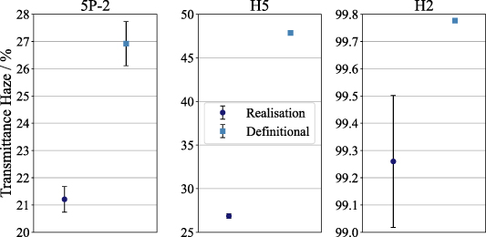
Figure 9. Haze values measured according to the definition, using integrated BTDF data, compared with realisation haze values measured using the integrating sphere according to the CMS method [8]. The error bars plotted show the expanded uncertainties calculated as 95% confidence intervals.
Download figure:
Standard image High-resolution imageConsidering the integrating sphere geometry, this is to be expected. In the integrating sphere measurements, the diffuse transmittance measurement includes all the light that is not lost through the exit port. Since a source of finite extent is used, the scattering angles of the light lost through the exit port differ for different parts of the incident beam. For a ray centred on the entrance port, the diffuse transmittance measurement includes only light scattered by more than 4∘, while for a ray at the edge of the incident beam, the diffuse transmittance measurement includes some light scattered by only 1.3∘. Therefore, the difference between the realisation haze and the definitional haze depends on the shape of the BTDF in this range of angles.
By changing the cut-off angle that the diffuse transmittance measurement is integrated from, the angle required to obtain the sphere haze value can be determined. For the H2 sample, this angle is 5∘, while for the 5P-2 and H5 samples, the angle is 3.5∘. Therefore, the disagreement between the sphere haze and the definitional haze cannot be resolved by changing the angle specified in the definition, as the angle depends on the sample.
5. Simulating sphere haze
Measurements of the BTDF can also be used to simulate the haze that would be measured by an integrating sphere. This can be done using ray tracing, by dividing the incident beam into rays, then for each ray, assuming it would be scattered according to the measured BTDF, calculating the scattering angles that would be captured by the sphere and summing up the appropriate parts of the BTDF to simulate the integrating sphere haze.
For each ray, the parts of the BTDF that fall within the exit port are summed up. For each measured θd, the fractional overlapping area between the exit port and an annulus centred on θd was determined. Then, the solid angle subtended by this area from the entrance port was calculated. This was used to weight the measured flux per solid angle from the BTDF measurements. This was repeated for each measured θd overlapping the exit port and all the contributions were summed up. The haze could then be calculated by dividing the sum by the total transmittance. This was repeated for each ray in the extended source used for the sphere measurements and normalised by the number of rays.
The simulated haze values have been plotted in figure 10 along with the realisation haze from the integrating sphere measurements. The simulated values for the three samples all agree with the sphere measurements within the expanded uncertainties. An uncertainty budget for the realisation, definitional, and simulated haze of the H5 sample has been included in the

Figure 10. Simulated integrating sphere haze values compared to the realisation haze values measured using the integrating sphere according to the CMS method [8]. The error bars plotted show the expanded uncertainties calculated as 95% confidence intervals.
Download figure:
Standard image High-resolution image5.1. Sphere geometry sensitivity
Simulating the integrating sphere haze in this way opens up several options for investigating the sensitivity of the realisation haze to different parameters that are difficult to physically vary in an instrument. For example, by varying the incident beam diameter or the exit port diameter in the simulations, the sensitivity of the sphere haze to the sphere geometry and alignment can be calculated. This could then lead to more robust uncertainty estimates of the haze measured in an integrating sphere.
Figure 11 shows the calculated relative change in the sphere haze value as the angle subtended by the exit port changes for the three samples, and figure 12 shows the relative change in the sphere haze value as the angle that the incident beam subtends changes. Looking at the exit port sensitivities, we can see that H2 is insensitive to errors in the size of the exit port, the haze of 5P-2 decreases by 12% per degree as the angle subtended by the exit port increases, and the haze of H5 drops by over 30% per degree as the angle subtended by the exit port increases. This demonstrates that small errors in the sphere geometry can have a significant influence on the haze measurements of samples, with the size of the error induced in the sphere measurement dependent on the shape of the BTDF of the sample.

Figure 11. Sensitivity of the sphere haze measurements to changes in the exit port radius.
Download figure:
Standard image High-resolution image
Figure 12. Sensitivity of the sphere haze measurements to changes in the beam radius.
Download figure:
Standard image High-resolution image
Similarly to errors in the angle subtended by the exit port, the haze measurements of H2 are almost insensitive to changes in the angle subtended by the incident beam, the sensitivity of the haze of 5P-2 with respect to the angle subtended by the incident beam is about 5% per degree, and the sensitivity of the haze of H5 is more than 10% per degree. This means that if there is an error of 0.2∘ in the angle subtended by the incident beam, which corresponds to the tolerance of 0.1∘ for the annulus around the incident beam at the exit port specified in the documentary standards, then the error in the haze measurement would be more than 5% for the H5 sample. Since the sensitivity to the angle subtended by the incident beam differs between the different samples, the uncertainty in the measured haze due to uncertainty in the angle subtended by the incident beam is sample dependent, with both the H5 and 5P-2 samples having larger errors than the 0.6% suggested by the ASTM and ISO standards and the H2 sample having a much smaller error.
Therefore, samples with high sensitivity to errors in the exit port size, such as H5, could be used to calibrate the integrating sphere geometry to ensure it meets the specifications in the documentary standards by comparing simulated and measured values of transmittance haze. If the sphere geometry did not fit the specifications in the documentary standards, then the simulated and measured values would not agree. The simulated sensitivity coefficients could also be included in the haze measurement model to account for uncertainty in the sphere geometry.
6. Conclusion
Measurements of the realisation transmittance haze made using an integrating sphere according to the documentary standard have been compared to values of the definitional haze calculated by integrating BTDF measurements according to the definition given in the standards. We have demonstrated that the sphere-based realisation of haze does not agree with the measurements made in accordance with the definition. This problem cannot be rectified by updating the definition to specify a new cut-off angle because the cut-off angle required to make the two values agree is different depending on the sample and the shape of its BTDF. The impact this has on haze measurements differs for different types of samples, but the sphere measurements always exclude some light scattered to wider angles than in the definition. This means that for some industries, haze might not be the most appropriate measurand, particularly for those interested in eliminating light scattering. For these industries, measurement of clarity [14], which measures narrow-angle scattering, may be more appropriate.
Like many other quantities intended to correlate with a visual perception, transmittance haze is a reduction of the full scattering distribution of a material to a single quantity. Whether this particular reduction is suitable depends on the purpose of the measurement and the visual effect that is sought.
In the future, it would be interesting to get a better understanding of the information that the various users of haze measurements require. Then, if the current sphere-based methods of realising haze are not appropriate, new measurement methods could be developed to suit the purpose of the measurements.
Acknowledgments
This work was funded by the New Zealand government and has been done in the frame of the Project 18SIB03 BxDiff, that has received funding from the EMPIR programme co-financed by the Participating States and from the European Union's Horizon 2020 research and innovation programme.
Appendix:
Table 1 shows the uncertainty budget for the realisation, definitional, and simulated haze for the H5 sample. Note that not all components apply to each method of measuring the haze. The uncertainty budgets for the other two samples are similar.
Table 1. Uncertainty budget for the realisation, definitional, and simulated haze for the H5 sample. The uncertainties in this table are absolute standard uncertainties.
| Realisation (%) | Definitional (%) | Simulated (%) | |
|---|---|---|---|
| Alignment | 0.0042 |

| |
| Angle setting | 0.032 | 0.0081 | |
| Dark | 0.0055 | 0.20 | 0.15 |
| Detector uniformity | 0.054 |

| |
| Linearity | 0.000 27 | ||
| MC integration | 0.0016 | ||
| Noise | 0.0082 | 0.0072 | 0.0050 |
| Sample uniformity | 0.13 | 0.14 | 0.051 |
| Solid angle | 0.098 | 0.030 | |
| Sphere geometry | 0.018 | ||
| Sphere uniformity | 0.027 | ||
| Stability | 0.0027 | ||
| Stray light | 0.000 27 | 0.041 | 0.025 |
| Total | 0.14 | 0.27 | 0.16 |