

Abstract
We describe the near real-time transient-source discovery engine for the intermediate Palomar Transient Factory (iPTF), currently in operations at the Infrared Processing and Analysis Center (IPAC), Caltech. We coin this system the IPAC/iPTF Discovery Engine (or IDE). We review the algorithms used for PSF-matching, image subtraction, detection, photometry, and machine-learned (ML) vetting of extracted transient candidates. We also review the performance of our ML classifier. For a limiting signal-to-noise ratio of 4 in relatively unconfused regions, bogus candidates from processing artifacts and imperfect image subtractions outnumber real transients by ≃10:1. This can be considerably higher for image data with inaccurate astrometric and/or PSF-matching solutions. Despite this occasionally high contamination rate, the ML classifier is able to identify real transients with an efficiency (or completeness) of ≃97% for a maximum tolerable false-positive rate of 1% when classifying raw candidates. All subtraction-image metrics, source features, ML probability-based real-bogus scores, contextual metadata from other surveys, and possible associations with known Solar System objects are stored in a relational database for retrieval by the various science working groups. We review our efforts in mitigating false-positives and our experience in optimizing the overall system in response to the multitude of science projects underway with iPTF.
Export citation and abstract BibTeX RIS
1. Introduction
The Palomar Transient Factory (PTF; Rau et al. 2009) and its successor survey currently underway, the intermediate Palomar Transient Factory (iPTF; Kulkarni 2013) have been advancing our knowledge of the transient, variable, and dynamic sky at optical wavelengths since 2009 March. From new classes of supernovae (Maguire et al. 2014; White et al. 2015), identifying gamma-ray burst optical afterglows (Singer et al. 2015) and counterparts to gravitational wave triggers (Kasliwal et al. 2016), exotic stellar outbursts (Miller et al. 2011; Tang et al. 2014), Milky Way tomography (Sesar et al. 2013) to near-Earth asteroids (Waszczak et al. 2016) and comets (Waszczak et al. 2013), iPTF continues to deliver,8
serving as a testbed for the development of future time-domain surveys. iPTF uses a 92-megapixel camera mosaicked into eleven functional 2048 × 4096 CCDs covering 7.26 deg2 on the Palomar 48-inch Samuel Oschin Schmidt telescope. The single exposures reach a depth of (Mould) R ≃ 21 mag (5σ) in 60 s. The pixel scale is ≈1'' and the image quality is ≈2 2 (median FWHM), implying the Point Spread Function (PSF) is better than critically sampled slightly more than 50% of the time. Further details of the hardware, survey design, and on-sky performance are described in Law et al. (2009, 2010) and Ofek et al. (2012). An overview of the image pre-processing and photometry pipelines, and archival system is described in Laher et al. (2014).
The near real-time discovery of transients from iPTF imaging data is currently performed using an image differencing pipeline at the National Energy Research Scientific Computing Center (NERSC; Cao et al. 2016). New incoming images are astrometrically and instrumentally calibrated, then aligned, PSF-matched, and differenced with deeper reference images supplied by the Infrared Processing and Analysis Center (IPAC, Caltech; Laher et al. 2014). Transient candidates are extracted from the differenced images then vetted using a classification engine (Bloom et al. 2012; Rusu et al. 2014). The NERSC infrastructure has contributed immensely to the success of PTF and iPTF.
We have implemented an enhanced version of the discovery pipeline to complement the pipeline at NERSC. In 2017, the iPTF project will be replaced by the Zwicky Transient Facility (ZTF) using a new camera on the same telescope (Bellm 2014; Smith et al. 2014). The ZTF camera will have a field of view of ∼47 square degrees, enabling a full scan of the Northern visible sky every night, at a rate ∼15 times faster than iPTF to similar depths. The massive high-rate data stream and volume expected from ZTF will require advancements in algorithms and data-management practices despite the (inevitable) growth in hardware technology. This will pave the way to the Large Synoptic Survey Telescope (LSST; Ivezić et al. 2014) that is expected to yield at least 100× as many astrophysical transients per image exposure than ZTF. In anticipation of this data deluge, we have embarked on a new efficient discovery pipeline and infrastructure at IPAC. Our design philosophy is flexibility, i.e., being able to operate in a range of complex astrophysical environments (including the galactic plane), robustness to instrumental glitches, adaptability to a wide range of atmospheric seeing and transparency, minimal tuning (unless warranted by instrumental changes), optimality (in the signal-to-noise sense), reliability in extracted candidates to moderately low S/N levels, and fast delivery of vetted candidates to enable follow-up in near real-time.
Searches for astrophysical transients (by virtue of changes in flux and/or position) have traditionally been conducted using either of two approaches. The first involves differencing of astrometrically aligned, PSF-matched images from two epochs: the science or target image containing the potential transient sources, and a deeper reference or template image serving as a static representation of the sky, for example, defined from an average of images from multiple historical epochs. The difference image is then thresholded to find and measure excess signals, i.e., the transient candidates. This approach was (and in some cases continues to be) used by numerous synoptic surveys, e.g., OGLE (Wyrzykowski et al. 2014), ROTSE (Akerlof et al. 2003), La Silla-QUEST (Hadjiyska et al. 2012), Pan-STARRS (Kaiser et al. 2010), and PTF (Law et al. 2009). Although simple in theory, a challenging aspect of discovery via image differencing is the prior matching of PSFs between the input images. This has lead to an intensive, ongoing research effort (e.g., Alard & Lupton 1998; Alard 2000; Woźniak 2000; Bramich 2008; Yuan & Akerlof 2008; Becker et al. 2012; Bramich et al. 2016; Zackay et al. 2016). The ultimate goal is the elimination of systematic instrumental residuals, e.g., induced by non-optimal calibrations and/or PSF-matching upstream. These would otherwise contaminate lists of extracted transient candidates, i.e., the false positives that would need to be dealt with later (see below). In practice, one strives to minimize their occurence in difference images such that in a global sense, the resulting pixel fluctuations and photometric uncertainties of bona fide flux transients approach expectations from Poisson noise and/or detector read-noise.
The second approach involves positionally matching source catalogs extracted from images at different epochs and searching for large flux differences between the epochs, e.g., as used by the Catalina Real-time Transient Survey (CRTS; Drake et al. 2009). This method avoids systematics from color-correlated source-position misalignments due to differential chromatic refraction, an effect that can be severe for some facilities. However, this method requires a relatively large flux-difference threshold to ensure reliability. This is at the expense of a higher missed detection rate (incompleteness) at low flux levels, particularly in regions with a complex background and/or high source-density (e.g., the galactic plane) where positional-matching is a challenge. On the other hand, assuming optimally calibrated and instrumentally matched inputs, image differencing excels in regions where source confusion is high and/or where complex, fast-varying backgrounds are present (e.g., near or within galaxies). Due to its adaptability to a wide range of astrophysical environments, the PTF project adopted image differencing as its primary means for discovery.
Following the extraction of transient candidates from differenced images, a somewhat daunting problem is deciding which are bogus (i.e., spurious) or real and worthy of further study. The existing iPTF discovery pipeline at NERSC accomplishes this using a supervised machine-learned (ML) classifier (Bloom et al. 2012; Brink et al. 2013). Here, a pre-labelled training set of previously discovered real transients are first fit to a two-class (real or bogus) non-parametric model described by a number of selected source features (or metrics). This model is then used to predict the class (real or bogus) of future candidates according to some probability threshold. The probabilities are also referred to as RealBogus (or quality) scores.
The iPTF discovery pipeline at NERSC typically yields a few to ten real "interesting" transients per night (excluding Solar-System objects and periodic or reoccuring variables in regions with a high stellar density). For ZTF, we expect at least 100 such transients per night. Currently however, real iPTF transients can be outnumbered by spurious candidates (false positives) by more than two orders of magnitude, despite efforts to minimize their incidence through careful pre-calibration. The problem gets worse if one is interested in finding the rare gems down to low S/N levels (e.g., Masci 2012). Depending on the science goals, the vetted candidates need to be delivered in a timely manner to the respective science working groups for follow-up. At NERSC, this currently takes ∼30 minutes since observation. The goal is to get this below ∼15 minutes. Large numbers of false-positives can strain any machine-learned vetting process and affect its reliability (Brink et al. 2013). It is crucial that the vetting process be efficient and reliable.
We have developed an automated image-differencing, transient-extraction and vetting system at IPAC; hereafter, the IPAC/iPTF Discovery Engine (or IDE). This infrastructure is currently in use for iPTF and is expected to be a foundation for ZTF in future. We have 6+ years of PTF science data in hand (ongoing with iPTF) and an experienced team at NERSC that aided in developing and refining all aspects of a robust discovery engine—from instrumental calibration to vetted transient candidates. Guided by previous implementations of the image subtraction problem, this paper reviews our algorithms, optimization strategies, experiences, and liens. We also describe our probabilistic (real–bogus) classification scheme for vetting transient candidates, Quality Assurance (QA) metrics, and database (DB) schema.
We note that two of the core pipeline steps in IDE: (i) image-differencing (that includes pre-conditioning of image inputs), and (ii) extraction of raw transient candidates therefrom, are both implemented in a stand-alone software module called PTFIDE.9 In this paper, we use the acronym PTFIDE when referring to these specific processing steps, otherwise, we use IDE when referring to the overall processing system. The latter includes all pre-calibration steps (prior to PTFIDE), machine-learned vetting and archival steps (post-PTFIDE). Furthermore, when referring to astrophysical transients, we use the term "transient" in a generic sense, i.e., all types of flux-excesses that can be detected in difference images (in both the positive and negative sense, relative to a reference image template): moving objects, periodic or aperiodic variable sources, or short-lived (fast) events. The goal of IDE is to deliver reliable transient candidates to the various science working groups for further follow-up. From hereon, these science working groups will be referred to as "science marshals," or simply marshals.
This paper is organized as follows. In Section 2 we give an overview of IDE and provide references for more information on each subsystem, both in this paper and elsewhere. Section 3 gives a broad overview of the image differencing and extraction module PTFIDE and its dependencies: input parameters, reference-image building, and output products. Section 4 expands on the specific processing steps in PTFIDE: gain and background matching, astrometric refinement, reference-image resampling, and PSF-matching. This includes a summary of all image-based and transient-candidate source metrics, and their use in deriving simple initial quality scores. Section 5 reviews the DB schema for storing all difference image-based and source-based metrics. The machine-learned vetting infrastructure, which includes training, tuning, and its overall performance is described in Section 6. Lessons learned during the course of development and testing are given in Section 7. Future and potential enhancements are discussed in Section 8 and conclusions are given in Section 9.
2. Overview of the Near Real-time Discovery Engine
The raw camera-image files are first sent from the Palomar 48-inch Samuel Oschin Schmidt telescope to the San Diego Supercomputing Center via a ≈100 Mbit s−1 microwave link and then pushed to Caltech and IPAC over the internet (bandwidth is ≳1 Gbit s−1). At IPAC, the camera-image files are ingested into an archive and associated metadata are stored in a relational database for fast retrieval and processing soon thereafter (see below).
Figure 1 gives an overview of the near real-time discovery pipeline. An executive pipeline wrapper controls the various steps: preprocessing which performs basic instrumental and astrometric calibration per CCD image (light purple boxes); PTFIDE—the image-differencing and transient extraction module (red boxes); then returning to the pipeline executive for archiving, DB-loading, and machine-learned vetting (light purple boxes). The preprocessing steps are from a stripped down version of the PTF/iPTF frame-processing pipeline. This executes asynchronously and independently of IDE following ingestion of an entire night's worth of image data. The purpose of this pipeline is to provide accurately calibrated images and source catalogs for future public distribution. This pipeline and the IDE preprocessing steps borrowed therefrom (light purple boxes in Figure 1) are described in detail in Laher et al. (2014). Below we summarize the major processing steps. The steps specific to PTFIDE (red boxes) are expanded in Sections 3–6. Operational details and tools used by the various science marshals (green boxes) will be discussed in future papers. In particular, the streak-detection functionality that is designed to detect moving objects in difference images, i.e., that streak in individual exposures is described in Waszczak et al. (2016).

Figure 1. Processing flow in the near real-time IPAC/iPTF Discovery Engine (IDE). The color-coding separates the various modular steps: preprocessing, archival, and machine-learned vetting (light purple); core image-differencing and transient extraction module: PTFIDE (red); external science applications and follow-up marshals (green). See Section 2 for details.
Download figure:
Standard image High-resolution imageThe 92-megapixel raw camera-image files (one per exposure) are processed by the real-time pipeline soon after they are ingested, check-summed, and registered in the database at IPAC. The ingest process also loads a jobs database table that is automatically queried by the pipeline executive to initiate the camera-splitting pipeline (Laher et al. 2014). This pipeline splits the camera-images into twelve 17 MB CCD image files (with overscan regions included), and noting that one of the CCDs is defective. An initial astrometric solution is derived and attached to their FITS10 headers. This astrometric solution is not the final (and best) calibration attached to the CCD images prior to image-differencing with PTFIDE. It is used to support source-catalog overlays, quick-look image visualizations, and quality assurance (QA) from the archive. The individual raw CCD frames in FITS format are copied to a local sandbox directory and associated metadata (including quality metrics and image usability indicators) are stored in a database to facilitate retrieval for the next processing steps.
A number of preprocessing and instrumental calibration steps are then applied to the raw CCD image. These include a dynamic (floating) bias correction and a static bias correction, a flat-field (pixel-to-pixel responsivity) correction, and cropping to remove overscan regions. The static bias and flat-field calibration maps are retrieved from an archive. These are generally the latest (closest-in-time) products available for the night being processed, i.e., that were made by combining data from a prior night. For the flat-field calibration in particular, quality metrics are used to check that the responsivity pattern falls within the range expected for a specific CCD and filter. If not, a pristine superflat is used. This preprocessing also initiates and populates a 16-bit mask image to record bad hardware pixels for the specific CCD frame, badly calibrated pixels, and saturated pixels. This mask is further augmented below to record image artifacts and object detections.
At this stage, we have a bias-corrected, flattened CCD image and accompanying mask image. Sources are then extracted from the CCD image using SExtractor (Bertin & Arnouts 1996; Bertin 2006a) primarily to support astrometric calibration—the most important calibration step in the real-time pipeline since its accuracy is crucial to attaining good quality difference images (Section 4.2). The SExtractor module is executed twice. The first run is to compute an accurate value of the overall image seeing (point-source FWHM) from the mode of a filtered distribution of individual source FWHM values. This estimate is then used to support source-detection in the second SExtractor run via a point-source matched filter. The first SExtractor run also folds in the object detections into the image mask, or rather the contiguous pixels contributing to each object above the specified threshold. The createtrackimage module is also executed to detect satellite and aircraft tracks in the CCD image and record their locations in the image mask. These occur with a frequency of typically several times per night and the same track can cross multiple CCDs. Metrics for each track are also computed (e.g., length and median intensity) and stored in a database table. For details on track identification and characterization, see Laher et al. (2014). The second SExtractor run generates a source catalog for input into the astrometric calibration step.
Astrometric calibration is initially performed using SCAMP (Bertin 2006b, 2014). SCAMP is executed using one of two possible astrometric reference catalogs as input: if the CCD image overlaps entirely with a field from the Sloan Digital Sky Survey (SDSS), the SDSS-DR9 Catalog (Ahn et al. 2012) is used; otherwise, the UCAC4 Catalog (Zacharias et al. 2013) is used. If SCAMP fails to find an astrometric solution using either of these catalogs, it is rerun with the USNO-B1 Catalog (Monet et al. 2003). In addition to solving for the standard World Coordinate System (WCS) first-order terms (for a gnomonic sky-projection; Calabretta & Greisen 2002), SCAMP simultaneously solves for field of view distortion using the PV polynomial convention on a per-image basis. The solution implicitly captures both the fixed camera-distortion and any variable atmospheric refraction effects at the time of exposure. The WCS solution and PV distortion coefficients are written to the CCD image FITS header. To enable other downstream (as well as generic analysis) software to map from pixel to sky coordinates and vice-versa, the PV coefficients are converted to the SIP representation (Shupe et al. 2005) using the pv2sip module (Shupe et al. 2012). The associated SIP coefficients are also written to the FITS header.
The astrometric (and distortion) solution from SCAMP is then validated. The first validation step coarsely checks that the standard first-order WCS terms (pointing, rotation, and scale) are within their expected ranges according to specific prior values. The second validation step involves re-extracting sources from the astrometrically calibrated CCD image (again using SExtractor) and matching them to a filtered subset of sources from the 2MASS Point Source Catalog (PSC; Skrutskie et al. 2006). A matching radius of 2'' is used and a minimum of 20 2MASS matches must be present. If the number of matches exceeds this minimum, the axial root-mean-squared (rms) position differences are root-sum-squared (RSS'd) and compared against a threshold that is dependent on galactic latitude. This threshold (t) lies in the range  corresponding to galactic latitudes
  . The threshold is interpolated from a look-up table of predetermined values according to the galactic latitude of the input image. The reason for a latitude-dependent threshold is due to the less reliable rms estimates in position differences following source matching when the source density is high. We are less tolerant of larger rms estimates in this regime due to the higher probability of false matches.
If the above validation checks on the astrometry are not satisfied, another attempt is made at the astrometric calibration, this time by executing the Astrometry.net module (Lang et al. 2010). This module uses the 2MASS PSC as the astrometric-reference catalog. Astrometry.net also solves for distortion on a per-image basis, however, its representation is only in the SIP format. To ensure proper execution of other downstream pipeline modules that depend exclusively on the PV representation, the SIP coefficients are converted to PV equivalents using the sip2pv module (Shupe et al. 2012) and written to the FITS header. The solution from Astrometry.net is validated in the same manner as above using the 2MASS PSC. If the acceptability criteria are still not satisfied, a bit-flag is set in a database table for use downstream. Metrics to assess the astrometric performance on each image are computed and also stored in the database to facilitate future analysis and trending (for details, see Laher et al. 2014).
Figure 2(a) quantifies the astrometric performance of the real-time pipeline for 68,310 iPTF CCD images acquired from 2015 January 1 to 2015 May 1 that used the SDSS-DR9 Catalog in their SCAMP solution. This catalog covers ≃14,555 deg2 at galactic latitudes of typically  and has an overall astrometric accuracy (rms per axis) of ≃50 milli-arcseconds (mas) with respect to earlier UCAC releases (Pier et al. 2003). The median rms per iPTF CCD per axis is typically 115 mas with respect to SDSS-DR9. The astrometric performance outside the SDSS-DR9 footprint (calibrated using either UCAC4 or USNO-B1; see above) is similar, except however for exposures observed in regions with a high source-density (e.g., the galactic plane) where systematics are more prevalent. These systematics are currently being addressed since iPTF includes a number galactic-plane science programs. Figure 2(b) shows the rms distributions for a subset of 24,168 CCD images from the same SDSS-DR9 overlap region with respect to the 2MASS PSC. Here, only images containing >200 2MASS matches each were used. The median astrometric accuracy with respect to 2MASS degrades to ≃190 mas per axis. This larger rms is somewhat expected since the 2MASS PSC has an accuracy of typically 150–200 mas (Skrutskie et al. 2006).
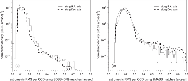
Figure 2. Distributions of the astrometric rms per CCD image along each axis with respect to (a) the SDSS-DR9 Catalog using 68,310 images and (b) the 2MASS PSC using a subset of 24,168 images containing sufficient matches. See the text for details.
Download figure:
Standard image High-resolution imagePreprocessing in the real-time pipeline also includes a step to detect and mask artifacts induced by bright-source reflections in the telescope optics, primarily ghosts and halos. The ghosts are due to bright sources lying off the telescope's optical axis, while halos are more coincident with the offending source. These features are located by first searching for bright (parent) stars from the Tycho-2 Catalog (Høg et al. 2000) with  mag. The positions of ghosts are then isolated using a pre-determined geometric mapping from the parent stars to expected ghost positions. Circular areas are flagged in the CCD bit-mask image to indicate probable ghosts and halos. Given the ghost and halo sizes vary with the brightness of the parent star, a conservative maximally sized masking area is used. The positions of ghosts, halos and their parent stars are stored in the database to facilitate future analysis. Lastly, the preprocessing phase computes a number of QA metrics for the image pixels and accompanying mask, a summary of which can be found in Laher et al. (2014). These are also loaded into the database.
There is no absolute photometric calibration in the preprocessing phase of the real-time pipeline to assign image-specific photometric zeropoints. Instead, the raw pixel signals are later throughput (gain)-matched to a reference image template during PTFIDE processing using sources extracted therefrom (Section 4.2). This reference image has an associated photometric zeropoint and therefore serves as the generic zeropoint for all real-time products that are matched to it, including the difference image products downstream. For details, see Sections 3.3 and 4.9.2. For an overview on the performance of the initial photometric calibration of the CCD images (on which the reference and difference-image products ultimately depend), see Ofek et al. (2012).
Figure 3 shows the typical durations of the primary steps in the real-time pipeline: from acquisition of a camera exposure to vetted candidates, ready to be examined by the science marshals. The median total time lag since exposure acquisition (Figure 3(b)) is ≃16 minutes and the 95th percentile is ≲22 minutes. When broken down into the various steps, the bulk of the lag is in the transfer of image data from the telescope to IPAC (≃9 minutes). This includes database ingestion and archiving, which amount to no more than several seconds per camera exposure. The preprocessing, PTFIDE and final archival steps amount to no more than ≃7 minutes, although there is a long tail in the PTFIDE runtime which we attribute to the extraction and processing of transient candidates from "bad" difference-images, i.e., containing an excess of residual artifacts (Section 6.2). The timing metrics shown in Figure 3 are those inferred at the time of writing using 1340 camera-image files and all eleven CCD images therein. The overall lag is expected to decrease in the near future, in particular in the transfer of image-data from the telescope to IPAC.

Figure 3. (a) Distributions of the elapsed time for various processing steps in the (near-)real-time discovery engine per CCD image. (b) Total elapsed time from acquisition of a CCD image exposure to vetted candidates extracted therefrom. Metrics were derived using 1340 camera-image exposures.
Download figure:
Standard image High-resolution imageAt the time of writing (pertaining to iPTF operations), the IDE pipeline executes on a Linux cluster of 23 machines consisting of 232 64-bit physical CPU cores in total: 11 machines have 8 Intel® Xeon® cores running at 3.0 GHz each and the remaining 12 machines have 12 similar cores running at 2.4 GHz each. All the machines, file and database servers are connected by a 10 Gbit network. Given that the 12-core machines can admit two threads per core, this cluster can in principle allow for 376 concurrent processes. However, since much of the processing involves a considerable amount of disk I/O, we achieve close to maximum throughput with only one thread per physical core, and therefore we usually execute at most 232 simultaneous threads. As raw camera-image files are received during the night, multiple instances of the camera-splitting pipeline are first run across all idle processor cores (until filled) to generate the individual raw CCD-images. These images then enter the processing queue and the level of core-parallelism now occurs at the CCD-image level through all the remaining pipeline steps (Figure 1).
The IDE pipeline was designed to be flexible enough to also process archival (preprocessed) image data. This mode facilitates pipeline tuning, iterative training of machined-learned classifiers in response to changing detector properties and/or science goals, but it also supports archival research in general, i.e., ad-hoc discovery projects using different pipeline parameters and thresholds. This offline execution mode only runs the PTFIDE steps (red boxes in Figure 1) using preprocessed image data that were previously instrumentally calibrated and archived by the regular PTF/iPTF frame-processing pipeline (Laher et al. 2014). This is because the preprocessed intermediate products from the initial phase of the IDE pipeline (light purple boxes in Figure 1) are not stored in a long-term archive.
To summarize, we have given a general overview of the near real-time IDE pipeline, with particular emphasis on the preprocessing steps needed to generate instrumentally and astrometrically calibrated CCD-images for input into the image-differencing and transient extraction module (PTFIDE). The primary outputs from the preprocessing step are a calibrated science image exposure, an accompanying bit-mask image, and metrics that quantify the astrometric performance and quality of the image-pixel data. The details on how these metrics and products are used in PTFIDE are discussed in Section 4.
3. PTFIDE Module Overview and Preliminaries
This section gives a broad overview of the PTFIDE software,11 dependencies, design assumptions, input data and formats, tunable parameters, and outputs—both primary products for archival and ancillary products for debug and analysis. PTFIDE is a standalone Unix command-line tool written in Perl. It calls a number of software executables written in C, C++ and Fortran. For a summary of the dependencies, see Section 3.1. The software can be built and configured to run under most Linux or Unix-like operating systems.
Figure 4 summarizes the main processing steps in PTFIDE, from preparing the inputs, to extracted transient candidates and metrics ready for loading into a relational database. A summary of all input files, parameters, and their default values is given in Section 3.2. One of the most important inputs is the reference image and its accompanying source catalog. Requirements regarding its construction are given in Section 3.3. Output products, formats, and their level of importance are summarized in Section 3.4. The details of each computational step in Figure 4 are expanded in Section 4.
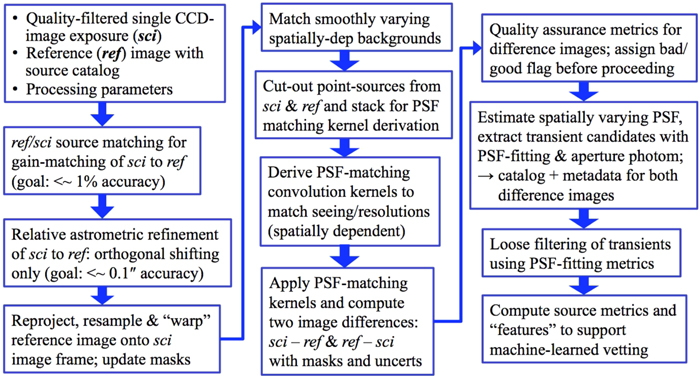
Figure 4. Processing flow in the PTFIDE (image differencing and extraction) module. These steps are contained in the first red box of the real-time pipeline flowchart in Figure 1. See Section 4 for details.
Download figure:
Standard image High-resolution image3.1. Software Design Philosophy, Dependencies, and Parallelization
To expedite the delivery of science quality products following the commencement of iPTF, some of the processing steps in PTFIDE leverage existing astronomical software tools. This is mostly heritage software that has been well tested by the astronomical community and refined over time. Table 1 summarizes the external (third-party) software components used in PTFIDE and other dependencies.
Table 1. External (Third-party) Software used by PTFIDE
| Software or Library | Versiona | Purpose |
|---|---|---|
| Perl |

|
Core language for scripting and performing arithmetic operations |
| PDL |

|
Perl module for vectorized image processing; built with bad-value and GSL support |
| GSL |

|
GNU Scientific Library (numerical library) |
| Astro-WCS-LibWCS |

|
Perl module to support World Coordinate System (WCS) transformations |
| Ptfutils, Pars | 1.0 | In-house developed Perl modules specific to PTF data processing |
| xy2xytrans | 2.0 | For fast image-to-image pixel position transformations |
| libtwoplane | 1.0 | Library to support xy2xytrans module |
| wcstools |

|
Contains WCS library to support multiple modules listed here |
| cfitsio |

|
FITS file-manipulation library to support multiple modules listed here |
| SExtractor | 2.8.6 | For initial source extraction to support internal source-matching steps |
| SWarp | 2.19.1 | For image resampling and interpolation using WCS |
| DAOPhot | II, 1/15/2004 | Source detection, aperture photometry, and PSF-estimation |
| Allstar | II, 2/7/2001 | PSF-fit photometry and support for PSF-estimation (included in DAOPhot package). |
Note.
aVersion number shown is that in use at the time of writing.Download table as: ASCIITypeset image
One of the design goals was robustness against missing or corrupted input data with appropriate error handling and reporting upon pipeline termination. Depending on the error, any missing (or out-of-range) data or associated metadata are replaced with default values in an attempt to salvage as many products as possible. Warnings are issued and logged if these occur. Furthermore, different pipeline exit codes are assigned according to the different anomalies (fatal and benign) encountered in processing. These status codes are stored as a bit-string in a database table to enable follow-up or to avoid querying unusable (or non-optimal) science products in future. Another design consideration was the ability to generate as many intermediate products and write as much information as possible from each processing step (Section 3.4). This was to facilitate offline debugging and tuning since many of the steps have complex interdependencies. This debug mode is controlled by a command-line switch and is typically turned off in operations to minimize runtime.
The base language in PTFIDE is Perl. This code executes both the external software modules and performs its own image-processing computations through use of the Perl Data Language (PDL; Glazebrook & Economou 1997). PDL is an object-oriented extension to Perl5 that is freely available as an add-on module. PDL is optimized for computations on large multidimensional data sets by making use of the hyper-threading capabilities of modern processor technologies. That is, PDL has its own threading engine that uses constructs from linear algebra to process large arrays as efficiently as possible using parallel computations. This is crucial since most of the steps in PTFIDE are CPU-bound. This low-level parallelism occurs on the individual processor cores where our basic processing unit is a single CCD-image. A higher level of parallelism is achieved by using all of the 232 CPU cores in our Linux cluster (described in Section 2). Here we typically execute 232 simultaneous threads (one CCD-image per core at any time). This gives us close to maximum throughput.
3.2. Primary Inputs and Parameter Summary
PTFIDE is driven by the Perl script ptfide.pl. The inputs can be broadly separated into the following: an instrumentally calibrated CCD-image exposure (the science image); an accompanying bit-mask (pixel-status) image; a spatially overlapping reference image; an accompanying source catalog for the reference image; configuration files for the various external software modules; processing parameters, thresholds, and control switches.
All image files are in FITS format (defined in Section 2). Input parameters and thresholds may be supplied on either the ptfide.pl command-line or in a configuration file, while image FITS-file names, other configuration files, and switches can only be supplied on the command-line. Table 2 summarizes the inputs to ptfide.pl with a brief explanation for each. The default parameter values are those currently used for iPTF. More details on some of the parameters can be found in Section 4.
Table 2. Inputs to PTFIDE (Script ptfide.pl)
| Inputa | Defaultb | Purposec |
|---|---|---|
| -cfgide | ⋯ | Optional input configuraton file listing all numerical parameters and thresholds defined below; these override those on the command-line, if any |
| -scilst | ⋯ | Input filename listing science image FITS file(s) |
| -msklst | ⋯ | Input filename listing mask image FITS file(s) accompanying -scilist |
| -ref | ⋯ | Input FITS filename of reference image (co-add) |
| -catref | ⋯ | Input reference image source catalog file from SExtractor; -cn specifies required columns |
| -cn | 2, 3, 4, 42, 10, 57, 60, 63, 72, 78, 27, 48, 14, 15, 45 | List of integers defining locations of required columns in the -catref input file |
| -catfilt | 0.5, 100, 19.0, 1.3 | Thresholds for filtering reference source catalog: min/max tolerable values for CLASS_STAR, ISOAREAF_IMAGE, MAG_APER, and ratio AWIN_WORLD/BWIN_WORLD |
| -od | ⋯ | Directory name for output products (including any debug output) |
| -cfgswp | ⋯ | Input configuration file for SWarp module |
| -cfgsex | ⋯ | Input configuration file for SExtractor to support position/gain matching |
| -cfgsexpsf | ⋯ | Input configuration file for SExtractor to support association with PSF extractions |
| -cfgcol | ⋯ | Input SExtractor column name configuration file to support position/gain matching |
| -cfgcolpsf | ⋯ | Input SExtractor column name configuration file to support association with PSF extractions |
| -cfgfil | ⋯ | Input filename for SExtractor convolution kernel filter |
| -cfgnnw | ⋯ | Input SExtractor neural network configuration file for star/galaxy classification |
| -cfgdao | ⋯ | Input generic DAOPhot parameter file |
| -cfgpht | ⋯ | Input DAOPhot photometry parameter file |
| -tmaxpsf | 2000.0 | Threshold [#bckgnd sigma] above background in reference image for maximum usable pixel value when creating PSF |
| -tdetpsf | 50.0 | DAOPhot findthreshold [#bckgnd sigma] for PSF creation from reference image |
| -tmaxdao | 3000.0 | Threshold [#bckgnd sigma] above zero-background in difference image for maximum usable pixel value for source extraction |
| -tdetdao | 3.5 | DAOPhot findthreshold [#bckgnd sigma] for source extraction on difference image |
| -tchi | 8.0 | Threshold on chi metric from Allstar program below which extractions on difference image are retained; larger  more non-PSF-like profiles are retained more non-PSF-like profiles are retained |
| -tshp | 4.0 | Threshold on sharp metric from Allstar program where extractions on difference image with –tshp  +tshp are retained; values of sharp ≃ 0 +tshp are retained; values of sharp ≃ 0  sources are more PSF-like sources are more PSF-like |
| -tsnr | 4.0 | Threshold on flux signal-to-noise ratio in PSF-fit photometry above which difference image extractions are retained |
| -fatbits | 8, 9, 10, 12 | Fatal bits to mask as encoded in input mask images (-msklist input); set to 1 for no masking |
| -satbit | 8 | Saturation bit# in mask images for determining saturation level in science images |
| -expnbad | 3 | Mask an additional (expnbad × expnbad) - 1 pixels around each input masked science and reference image pixel; provides more complete blanketing |
| -eg | 1.5 | Native electronic gain of detector [e-/ADU]; used for pixel-uncertainty estimation |
| -sxt | 2.0 | SExtractor detection threshold [#sigma] to support position/gain matching |
| -rad | 3.0 | Match radius [pixels] for associating reference and science frame extractions for position refinement and gain matching |
| -nmin | 200 | Minimum number of reference-to-science image source matches above which to proceed with position refinement and gain matching |
| -dgt | 1.5 | Minimum relative gain factor [%] above which to proceed with relative gain correction |
| -dpt | 0.07 | Minimum offset [pixels] above which to proceed with position refinements (dX or dY) |
| -dgsnt | 5.0 | Minimum S/N ratio in gain factor above which to proceed with relative gain correction |
| -dpsnt | 5.0 | Minimum S/N ratio in deltas above which to proceed with position corrections (dX or dY) |
| -gridXY | 4,8 | Number of image partitions per axis to support differential SVB computation |
| -tpix | 2.0 | Threshold t [#sigma] for replacing pixel values > mode + t∗sigma in an image partition to support differential SVB computation |
| -tmode | 500.0 | Threshold t [%] for replacing all pixels of a partition with global mode if its local mode is ![$\gt (1+t[ \% ]/100)$](https://content.cld.iop.org/journals/1538-3873/129/971/014002/revision1/paspaa443cieqn14.gif) ∗ global mode; to support differential SVB computation ∗ global mode; to support differential SVB computation |
| -tsig | 100 | Threshold t [%] for replacing all pixels of a partition with local mode if its robust sigma is  t[%]/100) ∗ "median of all partition sigmas"; to support differential SVB computation t[%]/100) ∗ "median of all partition sigmas"; to support differential SVB computation |
| -rfac | 16 | Image-pixel sampling factor to speed up filtering for differential SVB computation |
| -szker | 41 | Median-filter size for downsampled image to support differential SVB computation [pixels] |
| -ker | LANCZOS3 | Interpolation kernel type for SWarp module |
| -zpskey | IMAGEZPT | Keyword name for photometric zeropoint in science image FITS headers |
| -zprkey | IMAGEZPT | Keyword name for photometric zeropoint in reference image FITS header |
| -pmeth | 2 | Method to derive PSF-matching kernel between sci and ref images: 1  old Alard & Lupton (1998) method (now deprecated); 2 old Alard & Lupton (1998) method (now deprecated); 2  Pixelated Convolution Kernel (PiCK) method Pixelated Convolution Kernel (PiCK) method |
| -conv | auto | For -pmeth 2: image to convolve; can be sci, ref, or auto. The auto option uses the sci and ref FWHM values to select the image to convolve |
| -kersz | 9 | For -pmeth 2: linear size of PSF-matching kernel stamps [pixels] |
| -kerXY | 3,3 | For -pmeth 2: number of image partitions along X, Y to represent spatially dependent kernel |
| -psfsz | 25 | For -pmeth 2 if -rpick was set: linear size of PSF stamps created from point source cutouts |
| -apr | 9.0 | For -pmeth 2 if -rpick was set: source aperture radius [pixels] to compute flux for normalizing PSFs and background level outside this |
| -nmins | 20 | For -pmeth 2 if -rpick was set: minimum number of sources in an image partition above which PSF-creation is attempted |
| -nmaxs | 150 | For -pmeth 2 if -rpick was set: use n brightest sources per image partition for PSF-creation |
| -rpickthres | 4.0, 5.0, 0.0004, 40, 0.045 | For -pmeth 2 if -rpick was set: list of parameter thresholds for creating PSFs: N-sigma threshold for stack-outlier rejection; N-sigma threshold for spatial outlier-detection and winsorisation; maximum tolerable RSS of spatial RMSs of PSF products for (re)assigning partition inputs for kernel derivation; minimum distance to edge to avoid when selecting sources from sci and ref images; threshold td for  where R = ratio of PSF pixel sums and PSFs with where R = ratio of PSF pixel sums and PSFs with  are rescaled to the median{R} of all image partitions are rescaled to the median{R} of all image partitions |
| -nbreftb | 65 | For -pmeth 2: number of pixel rows to force as bad at top and bottom of internal images used for kernel derivation to account for edge effects in resampled reference image |
| -nbreflr | 35 | For -pmeth 2: number of pixel columns to force as bad at left and right of internal images used for kernel derivation to account for edge effects in resampled reference image |
| -bckwin | 31 | For -pmeth 2: linear window size for median filtering of [downsampled] reference image when computing spatially varying background; note: downsampling factor is fixed at 16× per axis |
| -tsat | 0.65 | For -pmeth 2: factor threshold to perform more conservative tagging of resampled ref image pixels satisfying  where where  and saturate is from resampled ref image header. This assumes the ref image was made using the mkcoadd.pl co-addition software and saturate is from resampled ref image header. This assumes the ref image was made using the mkcoadd.pl co-addition software |
| -goodcuts | 5.3, 1.2, 5.0, 0.02, 22, 4, 0.8, 35, 14.3, 7.0, 2, 0.07, 0.2 | For -pmeth 2: list of parameter thresholds for performing simple 1D cuts on source metrics for assigning goodcand flag in output extraction tables: chi, sharp, snrpsf, magfromlim, nneg, nbad, magdiff, mindtoedge, magnear, dnear, elong,  , kpr , kpr |
| -baddiff | 80, 15, 15, 3, 140, 0.2, 0.7, 0.15, 0.15, 1.5, 1.5 | List of parameter thresholds for performing simple 1D cuts on difference-image metrics for assigning good flag in output QA file: diffpctbad, dmedchi, davgchi, diffsigpixmin, diffsigpixmax, dmedksum, medkpr, ncandscimrefratio, ncandrefmsciratio, dinpseeing, dconvseeing |
| -uglydiff | 80, 15, 15, 140, 0.2, 0.7, 0.35 | List of parameter thresholds for performing simple 1D cuts on difference-image metrics to decide if should proceed with source extraction on difference images: diffpctbad, dmedchi, davgchi, diffsigpixmax, dmedksum, medkpr, maxminksum |
| -qas | 41, 2008, 41, 4056 | Coordinate range of rectangular region in image for computing QA metrics in difference images if -qa switch was set; format is: xmin, xmax, ymin, ymax where pixel numbering is unit based and  
|
| -apnum | 3 | Internal aperture number for which DAOPhot aperture photometry information should be propagated to output PSF-fit photometry table |
| -forceparams | R.A., decl., 43 | List of parameters to support "forced sub-image mode" if -forced switch was set; parameters are: R.A. [deg], decl. [deg], linsize [pixels] |
| -kerlst | ⋯ | Input filename listing FITS image cubes storing prior-derived, spatially dependent PSF-matching kernels for each science image to support "forced sub-image mode." |
| -phtcalsci | ⋯ | Switch to perform absolute photometric calibration of input science image after gain-matching to ref-image by computing a ZP using the calibrated MAG_AUTO values in the ref-image SExtractor catalog; this ZP will allow big-aperture (and PSF-fit) absolute photometry on the input science image before further gain refinements in the PSF-matching step downstream |
| -phtcaldif | ⋯ | Switch to perform absolute photometric calibration on science image after possible gain refinement and before image-differencing with ref-image by computing a ZP using the calibrated MAG_AUTO values in the ref-image SExtractor catalog; this ZP will allow big-aperture (and PSF-fit) absolute photometry on the science and difference images |
| -wmode | ⋯ | Switch to compute image modes (instead of medians) for the differential SVB correction |
| -rpick | ⋯ | Switch to use robust version of the PiCK method (-pmeth 2) when deriving PSF-matching kernel, i.e., via the construction of image PSFs using point-source cutouts |
| -psffit | ⋯ | Switch to perform PSF-fit photometry on difference images with prior PSF estimation off [possibly convolved] reference image |
| -apphot | ⋯ | Switch to perform fixed-aperture photometry on difference images using DAOPhot |
| -dontextract | ⋯ | Switch to only estimate spatially varying PSF; no extraction or photometry is performed |
| -forced | ⋯ | Switch to execute in "forced sub-image mode" where only "sci minus ref" difference image stamps (and ancillary files) centered on input R.A., decl. (-forceparams inputs) are made |
| -outstp | ⋯ | Switch to generate image cutouts of candidates from "sci minus ref" difference images |
| -pg | ⋯ | Switch to compute sci-to-ref relative astrometric and gain corrections, and apply if significant |
| -pcln | ⋯ | Switch to pre-clean (remove) output products directory specified by -od |
| -qa | ⋯ | Switch to generate QA metrics on difference images before and after PSF-matching within image slice defined by -qas string; results are written to standard output and an ASCII file |
| -d | ⋯ | Switch to write debug information to standard output, ASCII files and FITS images |
| -v | ⋯ | Switch to increase verbosity to standard output. |
Notes.
aThis same name (with prefix "–") is used in the ptfide.pl command-line specification. bDefault values, where shown, are optimal for the iPTF real-time pipeline. Command-line switches are "off" by default. cSome of these are further discussed in Section 4.3.3. Reference Image Construction and Requirements
The purpose of a reference image is to provide a static representation of the sky, or more specifically, a historical snapshot as defined by the state of the sky recorded in previous image exposures. This image provides a benchmark against which future exposures can be compared (i.e., differenced) to assist with transient discovery, both temporally (for flux changes) and/or spatially (for motion changes). The reference images also provide "absolute anchors" for assigning a photometric calibration to the incoming real-time science images and difference images derived therefrom. They are also used to check and refine astrometric solutions prior to differencing. Details are given below.
The reference images are co-adds (stack averages; see below) of several to fifty high-quality CCD-images selected from the image archive. Therefore, they have a higher S/N than the individual exposures. Besides supporting transient discovery, they can also benefit other science applications that require deeper photometry. So far in iPTF, the goal has been to construct reference images that are optimal for single-exposure image differencing and transient discovery. These do not necessarily achieve the highest possible depths (S/N) by using all available (good quality) images. This may be performed at a later date on completion of the survey and with different input image selection criteria.
Reference images are generated by a separate pipeline in iPTF operations that executes asynchronously and is independent of the real-time pipeline. This pipeline is only triggered when enough good quality images are available for a given field, CCD, and filter in the archive. The generation process is iterative in that reference images are remade and refined if an existing product is identified to be of low quality or unusable, provided better quality image-data are available. The input-image selection criteria for reference image generation were outlined in Laher et al. (2014). Given their importance, we repeat them below and expand on some of the details. These were derived from analyses of the distributions of numerous image metrics in 2013 June. The goal was to cover as much of the iPTF-visible sky as possible according to the available depth-of-coverage across all visited fields at the time.
- 1.The image must have been astrometrically and photometrically calibrated in an absolute sense and passed all automated quality checks prior to archiving (Laher et al. 2014).
- 2.The astrometric calibration (including full distortion solution) must have passed all validation steps (Section 2). This includes a separate check on the higher-order terms of the distortion polynomial.
- 3.The spatially binned photometric zeropoint values (provided by the ZP Variations Map or ZPVM from photometric calibration) must lie within ±0.15 mag. Furthermore, the source color-term coefficients derived from photometric calibration (as described in Ofek et al. 2012) must lie between the overall observed 1st and 99th percentiles.
- 4.The seeing (inferred from the mode of the point-source FWHM distribution) is
 .
. - 5.The 5-σ limiting magnitude, estimated using both theoretical and empirically derived inputs is mag.
- 6.The number of sources extracted from the image (via SExtractor) is. This reinforces the previous criterion and ensures the transparency was not too low or image noise not too excessive.
- 7.The minimum number of input images that must satisfy the above criteria before proceeding with reference image generation is Nmin = 5.


If  , the image limiting magnitudes Rlim are then sorted in descending order (faintest to brightest). Next, co-add limiting magnitudes mclim are predicted cumulatively and incrementally per-image for this list of candidate images. The resulting values of mclim are then compared to a predefined set of six target magnitude limits desired for the final co-add; e.g., for the iPTF R filter, these are defined:
where  , Rmedlim is the typical (median) 5-σ limiting magnitude of a single R-band exposure (Law et al. 2009), and Nmin = 5. The faintest target limit
  is then identified as the faintest mtlim that just falls below the co-add limit predicted from the entire image-list:
  . The number of images N to co-add is then the smallest possible N whose cumulative mclim comes closest to
  , i.e.,
where 50 is the maximum number of images allowed at this stage.
The requirement of an upper cutoff in the input image FWHM (36; criterion #4 above) is an important consideration since it influences the quality (effective point-source FWHM) of the resulting reference image and image subtractions derived therefrom. It is desirable to generate a reference image whose effective FWHM is smaller than that generally expected in the science (target) images. This ensures the higher S/N reference image is preferentially convolved (smoothed) to match the science image PSF prior to subtraction in PTFIDE. Not only will this minimize the relative fraction of correlated pixel-noise in the difference images (i.e., since noise will be dominated by the science image), it ensures robustness and minimizes the potential for error when using an automatic method to decide on which image to convolve. This is because the decision metrics themselves are inherently noisy and one cannot be confident that the correct image will always be selected. For the interested reader, Huckvale et al. (2014) present an analysis on ways to select the best reference image and convolution direction for optimal image subtraction in the presence of variable seeing. The median FWHM of the iPTF science images is ≈22. Therefore, it is inevitable that some cases will require the science image to be convolved when matching PSFs. This is not detrimental since PTFIDE can automatically select the image to convolve, with some margin for error (see below). The desire to have a lower cutoff for the input image FWHM when constructing reference images is mentioned here as a future improvement, specifically to optimize image subtraction. As mentioned, the requirement of FWHM  was driven by data availability (after accounting for all other selection criteria) and a need to generate reference images for a large fraction of the iPTF survey fields in short order.
Before co-addition to create a reference image, the input list of high-quality overlapping CCD-images (for a given field and filter) are astrometrically refined as an ensemble. This is performed in a relative image-to-image sense using SCAMP with inputs provided by SExtractor. Their distortion solutions (in the PV format) are also refined self-consistently. This improves the astrometric solutions of the input images as well as the overall astrometry in final co-adds.
Following astrometric refinement, the images are fed to an in-house developed co-addition tool (mkcoadd.pl) specifically written for iPTF. This software first determines the WCS geometry of the output co-add footprint using WCS metadata from all the input images. The co-add pixel scale is set to the native value determined for the center of the focal plane: 101/pixel, and the footprint X, Y dimensions are fixed at 2500 pixels × 4600 pixels throughout. These dimensions can accomodate for slight offsets in the reconstructed image pointing within a field. Retaining the native pixel scale for co-add images ensures they more-or-less remain (marginally) critically sampled in median seeing conditions. A future consideration would be to use half the native pixel scale to take advantage of the natural dithering offered by random offsets in telescope pointing across image epochs. This dithering would benefit input lists that are dominated by undersampled images (i.e., acquired in better than median seeing) so that the effective PSF can be better sampled when all images are combined.
Bad and saturated pixels are internally set to NaN in each CCD-image using their accompanying masks. This facilitates easier omission and tracking of all bad pixels downstream. Respective image-median levels are then subtracted. This stabilizes (or homogenizes) the images against temporally varying backgrounds before they are combined (see below). These backgrounds are not always astrophysical, for example, there is contamination from scattered moonlight and internal scattering from other bright objects whose line-of-sight may not directly fall on the focal plane. The individual image background levels are stored for later use. Each image is then de-warped (distortion-corrected) and interpolated onto the output co-add grid using its astrometric and distortion solution. This is accomplished using the SWarp software (Bertin et al. 2002). For an image observed at epoch t, the pixel values  at distortion-corrected positions i, j are interpolated and resampled using a 2D Lanczos kernel of window size three:

where  and
and  , and the signal at pixel position x, y in the output grid is given by
This generates a new set of images for epochs t = 1, 2, 3...N that have been corrected for distortion, all sharing the same WCS geometry, i.e., that of the final co-add footprint.
The choice of a Lanczos kernel (Equation (1)), particularly with window size three, is motivated by three reasons. First, it is close to optimal for PSFs that are sampled close to or above the Nyquist rate, i.e., its sinc-like properties can reconstruct well-sampled signals to good accuracy. By "optimal," we mean in the context of conserving information content. Second, its sinc-like nature also ensures that uncorrelated input noise remains close to uncorrelated on output. Third, its relatively compact support minimizes aliasing and the spreading of bad and saturated pixels on output. Given the ≈1'' pixel size, one small downside is that localized ringing can occur when the PSF is severely undersampled, i.e., when the seeing falls below ≈16.
Since the epochal images will have been observed at different atmospheric transparencies, their photometric throughput (or effective photon-to-DN gain factors) will be different. Throughput-matching the images to a common photometric gain or zeropoint (ZP) value is therefore necessary before combining them. This can be done in a relative sense (by computing source-flux ratios across images and rescaling pixel values therein) or in an absolute sense using the image-ZP values derived from photometric calibration upstream. We have chosen to use the absolute ZP values to compute the gain-factors. This is accomplished by throughput-matching all images to a common target zero point of ZPc. This value becomes the final co-add (reference image) ZP, where currently, all archived PTF reference images have ZPc = 27 magnitudes. The gain-corrected pixel values in a resampled image at epoch t with specific zero point ZPt are given by

The resampled and throughput-matched epochal images with pixel signals  are then combined using a lightly-trimmed weighted-average. Outlier-trimming is performed on the individual pixel stacks (along the t dimension) by first computing robust measures of the location and spread: respectively the median (p50) and
 ![$\sigma \simeq 0.5[{p}_{84}-{p}_{16}]$](https://content.cld.iop.org/journals/1538-3873/129/971/014002/revision1/paspaa443cieqn38.gif) , where the px are percentiles. Pixels that satisfy
, where the px are percentiles. Pixels that satisfy  are rejected from their temporal-stack at position x, y prior to combining the remaining pixels using a weighted-average (see below). Our choice of a relatively loose trimming threshold (9σ) is driven by our goal to remove the largest outliers only (e.g., cosmic rays and unmasked satellite trails), therefore preserving as much information as possible.
The pixels in a stack are weighted using an inverse power of the seeing (FWHMt) in the images they originated from, i.e.,
where FWHM0 is a constant fiducial value currently set to the modal value of 2'' and is unimportant since it cancels following normalization in the final weighted average. α is a parameter that controls the overall importance of the weighting. This weighting is purely motivated by empirical and practical considerations as an attempt to handle the time-dependent seeing in a qualitative sense, i.e., in that relatively more weight is given to images acquired in better seeing. There is no theoretical justification that satisfies some optimality criterion like maximal S/N, however, it is interesting to note that α = 2 corresponds to the case where  , where Np is the effective number of noise pixels12
for a Gaussian-like PSF and
, where Np is the effective number of noise pixels12
for a Gaussian-like PSF and  is the flux-variance that would result from PSF-fit photometry on the image (see also Masci & Fowler 2009). Therefore when α = 2, the weighting is effectively inverse-variance weighting of the images according to the expected point-source flux uncertainties from PSF-fitting. Besides being optimal for PSF-fitting (simultaneously over the entire image stack), and particularly when the input noise is Gaussian, we found through simulation and analysis of on-sky data that α = 2 can lead to significantly distorted PSFs and slight degradations in the co-add pixel S/N. This is due to the undersampled nature of the PSF when the seeing is better than average in iPTF exposures. We found that values of
  for the range of seeing encountered (and a forced cutoff of FWHM
  see above) work best. As a compromise, we assumed α = 1 throughout. This choice is similar to that adopted by Jiang et al. (2014) for combining SDSS image data. These authors also included inverse-variance weights in their weighting scheme, with pixel variances computed from the background rms in each input image.
The Nr remaining pixels in a stack following outlier rejection are combined using a weighted average to produce the co-added pixel signal,
where  and wt are given by Equations (3) and (4) respectively. The Bct are the individual image background levels that were initially subtracted from each image (see above) then rescaled using the same throughput-match factors in Equation (3). A median of all these levels is computed and used as a fiducial background for the final co-add. We also generate an image of the uncertainties in the weighted averages S(x, y). For co-add pixel x, y, this can be written:
  where
where  and σt is the uncertainty (e.g., a prior) for the input pixel signal at x, y, t. We assume that the noise is spatially and temporally uncorrelated across images. Instead of using explicit priors for σt (e.g., from a pixel-noise model), we approximate σt using an unbiased and unweighted estimate of the population standard-deviation in the stack of
  values. The uncertainty in S(x, y) (Equation (5)) then becomes
The effective  scaling is implicitly represented by the fractional term involving wt. An image of the pixel depth-of-coverage, Nr(x, y), is also generated.
The astrometric solution in the reference image is validated against the 2MASS PSC using a procedure similar to that described in Section 2. Sources are extracted and measured from the reference image using both aperture (SExtractor) and PSF-fit photometry (DAOPhot). Ancillary products for the PSF-fit catalog include a DS9-region file and estimates of the spatially variable PSF represented in both DAOPhot's look-up-table format and as a grid of FITS-image stamps. QA metrics for the image and catalog products are also generated. The product files are archived and their paths/filenames and associated metrics stored in a relational database.
Each reference image product is uniquely identified according to survey field, CCD, filter, pipeline number, version, and archive status flag. The pipeline number supports variants of the reference image pipeline tailored for different science applications, for example, a specific time range, number of input images, and/or different filtering criteria than the default used to support real-time processing. As mentioned, the reference image library is periodically updated as low-quality or unusable products are identified from analyses of outputs from the real-time pipeline, provided enough good quality images are available (see above).
The reference image and its SExtractor catalog for a given survey field, CCD, and filter are two of the primary products used in PTFIDE (Section 4). As mentioned, these provide an absolute anchor for assigning a photometric ZP to all the new incoming, spatially coincident science images and subtractions derived therefrom. The ZP value in the FITS header of a reference image is the target fiducial value ZPc onto which selected input images were gain-matched prior to co-addition (Equation (3)). The absolute accuracy of ZPc is therefore determined by the accuracy of the input image ZPt values. These were initially derived from photometric calibration in the frame-processing pipeline using the SDSS-DR9 catalog (Ofek et al. 2012; Laher et al. 2014). The input instrumental magnitudes used to perform this calibration are Kron-like aperture measurements from SExtractor, also referred to as mag_auto. At the time of writing, these are the only instrumental magnitudes in iPTF products that can be tied to an absolute photometric system via the image ZPt values. The individual (spatially averaged) image ZPt values are accurate to 2%–4% (absolute rms; Ofek et al. 2012). These could be less accurate on sub-image scales due to possible residual spatial variations in the instrumental response. The ZPt-inherent gain-match errors will propagate into the reference image pixel values following image rescaling (Equation (3)). These errors will only be captured by the empirical uncertainty estimates in Equation (6) (with its implicit  scaling) assuming no systematics in the ZPt derivations upstream. A future goal is to calibrate the ZPt values to better than 1%, preferably using PSF-fit photometry.
3.4. Summary of Output Products
PTFIDE output products are files that are generically named: InputImgFilename_type.ext where InputImgFilename is the root filename assigned to the CCD image following pre-calibration upstream (Section 2) and type.ext is a mnemonic for the type of PTFIDE product generated. The extension (ext) can be either fits (for FITS-formatted image), tbl for ASCII table in the standard IPAC format, psf for PSF file in DAOPhot's look-up-table format, reg for DS9 region-overlay file, log for logfile, or txt for other ASCII files.
Table 3 lists the primary PTFIDE products generated per CCD image. By "primary," these represent the products that are later used for real-time transient discovery and/or general archival science applications, for example, light-curve generation using forced-photometry on the difference images. The image, PSF, QA, and log files are copied to long-term storage and their paths/filenames registered in relational database tables. The table (tbl) files contain the extracted transient candidates and associated metrics (Section 4.9.5), one for the positive and another for the negative difference image. The metadata for each transient are later stored in database tables (see Section 5). The metrics in the _diffqa.txt QA files (Section 4.8.2) are stored in a separate database table. The generation of positive (sci—ref) and negative (ref—sci) difference images may seem somewhat redundant since one is simply the negative of the other. The purpose of having a negative difference is to enable detection of transients that dissapear below the reference image baseline level, for example, variable stars that are observed in their "low" state relative to their time-averaged (reference image) flux. Our source detection software is designed to detect positive signals only and therefore it is necessary to negate the positive difference image and extract any new transients (or excursions in variable flux) that happened to be below the reference level at that epoch.
Table 3. Primary Outputs from PTFIDE
| Output file suffixa | Format | Descriptionb |
|---|---|---|
| _pmtchscimref.fits | FITS imagec | Final PSF-matched "science minus reference" difference image |
| _pmtchscimrefpsffit.tbl | IPAC table | Table of extracted transient candidates with PSF-fit and aperture photometry, and source metrics corresponding to the _pmtchscimref.fits difference image |
| _pmtchscimrefpsffit.reg | ASCII | DS9 region/source-overlay file for all transient candidates in _pmtchscimrefpsffit.tbl |
| _pmtchrefmsci.fits | FITS imagec | Final PSF-matched "reference minus science" difference image |
| _pmtchrefmscipsffit.tbl | IPAC table | Table of extracted transient candidates with PSF-fit and aperture photometry, and source metrics corresponding to the _pmtchrefmsci.fits difference image |
| _pmtchrefmscipsffit.reg | ASCII | DS9 region/source-overlay file for all transient candidates in _pmtchrefmscipsffit.tbl |
| _pmtchdiffunc.fits | FITS imagec | Image storing 1-σ pixel uncertainties corresponding to the _pmtchscimref.fits and _pmtchrefmsci.fits difference images |
| _pmtchkerncube.fits | FITS cube | Image stamps of spatially dependent PSF-matching convolution kernels with metadata in header. Each plane of cube stores kernel image for a specific partition in input science image |
| _pmtchconvrefdao.psf | ASCII | File storing PSF template generated by DAOPhot from the kernel-convolved reference image. Only generated if the reference image was convolved to match the science image seeing (FWHM) |
| _resamprefdao.psf | ASCII | File storing PSF template generated by DAOPhot directly from the reference image, with no convolution. Only generated if the science image was convolved to match the reference image FWHM |
| _diffqa.txt | ASCII | File storing QA metrics on image-differencing process and statistics on number of transients extracted |
| _ptfide.log | ASCII | Log file storing processing diagnostics and verbose output. |
Notes.
aThis is also a mnemonic for the product type; see Section 3.4. bMore details are given in Section 4. cThe sizes of these image files are ≃34 MB each (2048 × 4096 pixels with 32 bits per pixel).Download table as: ASCIITypeset image
Table 4 lists the secondary or ancillary PTFIDE products that can be generated per input CCD image. These are diagnostic files to support offline analysis, debugging and tuning, and are not generated by the (real-time) production pipeline. They are generated in addition to the products in Table 3 if the debug (-d) switch was specified for ptfide.pl. Furthermore, some products are only generated when ptfide.pl is executed in sub-image mode (with the -forced switch; Section 4.10).
Table 4. Ancillary (Debug-Mode) Outputs from PTFIDE
| Output file suffixa | Descriptionb |
|---|---|
| _badmsksci.fits | Bad pixel mask for science image that includes spatially expanded bad pixels |
| _badmskref.fits | Bad pixel mask for reference image (mostly showing saturated regions) |
| _scisatpixels.fits | Image showing locations of only saturated pixels in science image |
| sx_ref_filt.tbl | Table of filtered sources from input reference-image SExtractor catalog to support gain-matching and position refinement |
| sx_ref_filt.reg | DS9 region/source-overlay file corresponding to sx_ref_filt.tbl |
| _sxrefremap.tbl | Table of positions and fluxes of filtered reference image sources from sx_ref_filt.tbl with positions mapped onto science image frame to support source-association in SExtractor run |
| _sx.tbl | SExtractor catalog of science image extractions matched to filtered and remapped reference image sources from _sxrefremap.tbl; to support gain-matching and photometric calibration |
| _sx.reg | DS9 region/source-overlay file corresponding to _sx.tbl |
| _sxbck.fits | Diagnostic background image computed by SExtractor when generating _sx.tbl catalog |
| _sxbckrms.fits | Diagnostic background rms image computed by SExtractor when generating _sx.tbl catalog |
| _sxobjects.fits | Diagnostic image showing objects extracted by SExtractor when generating _sx.tbl catalog |
| _resampref.fits | Reference image resampled onto science image frame |
| _resamprefunc.fits | Pixel-uncertainty image corresponding to _resampref.fits |
| _resamprefwt.fits | Weight image from resampling of reference image using SWarp |
| _newscitmp.fits | Science image gain-matched and positionally refined relative to reference image |
| _inpsvb.fits | Regularized image used to compute smoothly varying differential background (SVB) image |
| _svb.fits | Image of smoothly varying differential background; used to correct science image |
| _newscibmtch.fits | Science image with differential background, photometric gain, and astrometry matched to resampled reference image, before PSF-matching |
| _newsciuncbmtch.fits | Pixel-uncertainty image corresponding to _newscibmtch.fits |
| _diffbmtch.fits | Internal "science minus reference" difference image before any PSF-matching |
| _noconv_pm_stpn.fits | Point-source image stamp indexed by  in partition in partition  of image that is not convolved of image that is not convolved |
| _toconv_pm_stpn.fits | Point-source image stamp indexed by  in partition in partition  of image that will be convolved of image that will be convolved |
| _noconv_pm_psfcoad.fits | Final co-added PSF from all point-source stamps in partition  of image that is not convolved; used to derive PSF-matching kernel for partition of image that is not convolved; used to derive PSF-matching kernel for partition 
|
| _toconv_pm_psfcoad.fits | Final co-added PSF from all point-source stamps in partition  of image that will be convolved; used to derive PSF-matching kernel for partition of image that will be convolved; used to derive PSF-matching kernel for partition 
|
| _noconv_pm_psfcoaddepth.fits | Pixel depth-of-coverage map corresponding to _noconv_pm_psfcoad.fits |
| _toconv_pm_psfcoaddepth.fits | Pixel depth-of-coverage map corresponding to _toconv_pm_psfcoad.fits |
| _sxrefremapcorr.tbl | Equivalent to _sxrefremap.tbl but performed on regularized science image (gain-matched, position-refined, and PSF-matched with additional gain-corrections) prior to differencing |
| _scibefdiff.fits | Regularized science image (gain-matched, position-refined, and PSF-matched with additional gain-corrections); input for SExtractor to generate _sx_scibefdiff.tbl catalog |
| _sx_scibefdiff.tbl | SExtractor catalog of science image extractions matched to filtered and remapped ref image sources from _sxrefremapcorr.tbl; to support photometric calibration of difference image |
| _pmtchconvref.fits | Convolved reference image prior to differencing; only produced if ref image was convolved |
| _pmtchconvsci.fits | Convolved science image prior to differencing; only produced if sci image was convolved |
| _pmtchdiffmsk.fits | Bad-pixel mask for final difference images; includes effects of convolution from PSF-matching |
| _pmtchdiffchisq.fits | Image of binned pseudo-χ2 values for difference image after PSF-matching |
| _pmtchconvref.cooc | DAOPhot output file listing initial detections from _pmtchconvref.fits for PSF generation |
| _pmtchconvref.lstc | DAOPhot output file listing stars picked from _pmtchconvref.fits for PSF generation |
| _pmtchconvref.lst.regc | DS9 region/source-overlay file corresponding to_pmtchconvref.lst |
| _pmtchconvref.neic | Allstar/DAOPhot output file listing neighbors of the stars listed in _pmtchconvref.lst |
| _pmtchconvrefdaosub.fitsc | Allstar/DAOPhot output image showing PSF-subtracted sources from _pmtchconvref.fits |
| _pmtchconvrefdaopsf.fitsc | Image of spatially varying PSF represented as a grid of 16 × 32 postage stamps |
| _pmtchscimref.coo | DAOPhot output file listing initial detections from _pmtchscimref.fits difference image |
| _pmtchrefmsci.coo | DAOPhot output file listing initial detections from _pmtchrefmsci.fits difference image |
| _pmtchscimrefdaosub.fits | Allstar/DAOPhot output image showing PSF-subtracted sources from _pmtchscimref.fits |
| _pmtchrefmscidaosub.fits | Allstar/DAOPhot output image showing PSF-subtracted sources from _pmtchrefmsci.fits |
| _pmtchscimrefapphot.tbl | Table containing concentric aperture photometry for extracted transient candidates from the _pmtchscimref.fits difference image; only generated if the –apphot switch was set |
| _pmtchscimrefapphot.reg | DS9 region/source-overlay file for all sources in _pmtchscimrefapphot.tbl |
| _pmtchrefmsciapphot.tbl | Table containing concentric aperture photometry for extracted transient candidates from the _pmtchrefmsci.fits difference image; only generated if the –apphot switch was set |
| _pmtchrefmsciapphot.reg | DS9 region/source-overlay file for all sources in _pmtchrefmsciapphot.tbl |
| _pmtchscimrefsex.tbl | SExtractor catalog for _pmtchscimref.fits difference image to associate with PSF-fit extractions; used to assign source-shape metrics |
| _pmtchrefmscisex.tbl | SExtractor catalog for _pmtchrefmsci.fits difference image to associate with PSF-fit extraction; used to assign source-shape metrics |
| _pmtchconvscistamp.fitsd | Convolved sci image stamp prior to differencing; only produced if sci image was convolved |
| _pmtchconvrefstamp.fitsd | Convolved ref image stamp prior to differencing; only produced if ref image was convolved |
| _imgtoconvstamp.fitsd | Stamp image that is not convolved with PSF-matching kernel. Can be either sci or ref image |
| _imgnoconvstamp.fitsd | Stamp image that will be convolved with PSF-matching kernel. Can be either sci or ref |
| _msktoconvstamp.fitsd | Mask image stamp corresponding to _imgtoconvstamp.fits |
| _msknoconvstamp.fitsd | Mask image stamp corresponding to _imgnoconvstamp.fits |
| _uncscistamp.fitsd | Pixel-uncertainty image stamp corresponding to regularized science image |
| _uncrefstamp.fitsd | Pixel-uncertainty image stamp corresponding to regularized reference image |
| _pmtchkernstamp.fitsd | Image of PSF-matching kernel used to convolve image stamp; extracted from archival _pmtchkerncube.fits file. |
Notes.
aThis is also a mnemonic for the product type; listed in approximately the same order as generated by ptfide.pl, along with the primary products in Table 3. bMore details are given in Section 4. cOnly generated if the resampled reference image was convolved with the PSF-matching kernel, otherwise, the pmtchconvref filename string is replaced with resampref if the science image was convolved. dOnly generated in "forced" sub-image mode if the -forced switch was specified in processing; see Section 4.10.4. PTFIDE Processing Steps
The input pre-calibrated CCD images need to satisfy a number of criteria prior to processing through PTFIDE. These criteria use a number of quality metrics computed upstream during preprocessing (Section 2). Inputs that do not satisfy these criteria are expected to be of low quality and are not used for transient discovery. Instead, they are assigned a status flag (that is encoded into an overall processing bit-string at the end of processing) and stored in a database table for future reference. The criteria currently used to declare a CCD image as "good" and worthy for image differencing are as follows:
- 1.The seeing FWHM on the corresponding raw exposure image satisfies FWHM . Values of FWHM are also a good proxy for low atmospheric transparency. Over the course of iPTF, ≃0.04% of exposures are above this limit.
- 2.The calculation of the seeing FWHM used in (1) was based on a sufficient number of point sources and is not a NaN. The latter may occur due to bad inputs.
- 3.At least 500 sources were found by SExtractor for use in the astrometric calibration using SCAMP.
- 4.The WCS solution from SCAMP used source matches with the astrometric catalog.
- 5.The WCS solution could be derived using SCAMP with no errors or warnings. I.e., the astrometric calibration did not fallback to Astrometry.net.
- 6.At least 20 sources were matched with the 2MASS PSC for validating the WCS.
- 7.The axial rms position differences using the 2MASS matches are within the maximum tolerable value (which depends on galactic latitude; see Section 2).
- 8.The first-order WCS terms (pointing, rotation, and scale) are within range.
- 9.The higher-order terms of the distortion polynomial are within range.


Below, we expand on the processing steps outlined in the PTFIDE processing flow of Figure 4. This includes additional details not shown in this figure. The descriptions make extensive use of the input parameters and output products summarized in Tables 2–4.
4.1. Mask-creation and Bad-pixel Expansion
The input bit-mask image for the CCD science image is first AND'd with the fatal-pixel bit-string template specified by –fatbits. This identifies those pixels to omit from processing. To enable tracking downstream, these pixels are forced to NaN and all good (usable) pixels are reset to 1 in an internal image mask. This mask is then further processed and regularized by forcing an additional (N × N) − 1 pixels around each masked (NaN'd) pixel to also be bad, where N = input from –expnbad parameter. This provides more complete blanketing of bad pixel regions, e.g., for saturated sources in particular whose unmasked edges and associated bleed artifacts will lead to residuals in the difference images and hence unreliable extractions. This expansion operation is also performed on saturated pixels in the resampled reference image, i.e., following reprojection onto the science image frame (Section 4.3). These internal regularized science and reference image masks are propagated downstream. In debug mode, they can be written to FITS format with filename suffixes _badmsksci.fits and _badmskref.fits respectively.
Another reason for spatially expanding all bad input pixels is that both the reference image resampling and the later PSF-matching step that involves convolving one of the images (Section 4.7) will cause bad-pixel regions to implicitly grow. A forced expansion provides a more conservative blanketing that is matched in both images prior to subtraction. Both the science and reference image masks are later combined (following PSF-matching) to produce a final effective bad-pixel mask (_pmtchdiffmsk.fits) for both difference images: _pmtchscimref.fits and _pmtchrefmsci.fits. Furthermore, all bad pixels in the difference images are tagged with value −999,999.
4.2. Relative Gain-matching and Astrometric Refinement
Two important preprocessing steps are photometric throughput (or gain)-matching and a (possible) astrometric alignment of the science image with the reference image. As discussed in Section 3.3, the reference image provides an absolute anchor for assigning a photometric zeropoint (ZP) and a WCS to the final difference image products. The relative photometric and astrometric corrections are first derived and validated, and then only applied to the science image if found to be statistically significant. We describe each in turn below.
First, the input reference image catalog from SExtractor (–catref) is filtered to retain primarily isolated point sources using the following SExtractor-derived metrics: CLASS_STAR (minimum stellarity index); ISOAREAF_IMAGE (maximum effective isophotal area); MAG_APER (faintest magnitude based on a fixed 14-pixel diameter aperture); and the ratio AWIN_WORLD/BWIN_WORLD (maximum effective source elongation). The thresholds for these metrics are specified by the –catfilt input. Another requirement is that all sources be clean and uncontaminated with no bad SExtractor flags, i.e., FLAGS = 0. A 14-pixel diameter aperture is used so that integrated source fluxes are relatively immune to seeing variations for the range of seeing encountered. This choice however is not optimal for crowded fields (see below). An intermediate filtered reference image catalog is then generated with filename sx_ref_filt.tbl.
The source x, y positions in the filtered reference image catalog are then mapped into the coordinate frame of the science image using the xy2xytrans utility. The reason for this is to support efficient source-matching within SExtractor when run in source-association mode (below) since it only supports source-matching in x, y coordinates. A new intermediate catalog is made with filename suffix _sxrefremap.tbl that stores photometric information for the filtered reference image sources and with x, y positions in the WCS of the science image. It is not guaranteed that this WCS is correct; hence any possible astrometric errors will be reflected in the remapped x, y positions. These positions will be used below to refine the overall astrometry. SExtractor is then executed in source-association mode using the filtered and position-remapped reference catalog sources. This entails finding the nearest science image sources with S/N above input threshold –sxt and within a radial tolerance of –rad. A source-matched catalog table is generated (_sx.tbl) with an accompanying DS9 region file (_sx.reg). This table is used to derive the gain and astrometric corrections.
4.2.1. Gain and Astrometric Corrections
The relative photometric gain factor Dg is estimated using a median of the flux ratios of all Nm science-to-reference source matches, where all fluxes are based on a 14-pixel diameter aperture13 :
The uncertainty in Dg is estimated from the Median Absolute Deviation (MAD), appropriately rescaled for consistency with Gaussian statistics in the limit of large Nm, and further inflated by  to account for the fact that the median in Equation (7) is noisier than a mean:
Global position offsets along the x and y axes are also computed using medians of the source-position differences:
with uncertainties that are also based on the MAD estimator, similar to Equation (8). Note that these represent overall orthogonal offsets between the science and reference images, and do not account for possible spatially dependent offsets, for example, that would result from an erroneous distortion solution for the science image (as calibrated upstream; see Section 2). Recall that the reference-image pixels have already been corrected for distortion during the co-addition process (Section 3.3). Therefore, the assumption here is that the distortion solution is reasonably accurate over the CCD image, and that any systematics in the relative astrometry are purely global shifts along either x or y or both.
Furthermore, to gauge the spread in the Nm input flux ratios (Equation (7)) and position offsets (Equation (9)), 5th—95th percentile ranges are also computed for these quantities. A large spread in the flux ratios for example (relative to some expected nominal value) may indicate that the flat-fielding was inaccurate upstream. A large spread in the position offsets may indicate that the distortion calibration was inaccurate. These metrics are stored in a database table for trending.
The gain correction factor Dg (Equation (7)) is only used to rescale the science image pixel values to match those in the reference image if the following criteria are satisfied: the number of matches Nm from which it was derived exceeds –nmin; the quantity  exceeds –dgt; and its significance or S/N ratio,
  , exceeds –dgsnt. Similarly, the orthogonal position corrections
  are only applied to the science image WCS parameters if the following criteria are satisfied: the number of matches Nm also exceeds –nmin; either
  or
or  exceed –dpt; and their S/N ratios,
  or
or  , exceed –dpsnt. Note, since the
  are constant corrections (independent of position), it suffices to simply correct the coordinate origin defining the science image WCS. These are the FITS keyword values CRPIX1 and CRPIX2, and are corrected to the new values
  and
and  respectively. This adjustment then ensures that the reference image is reprojected (and registered) onto the correct science image WCS later on (see Section 4.3).
As a detail, there are occasions when the input science image was already absolutely photometrically calibrated and associated with a ZP value, for example, when PTFIDE is executed in offline mode on processed archival data. In this case, an initial global gain correction factor G is computed using the science and reference image ZP values according to Equation (3). The Dg factor (Equation (7)) is still computed, but it becomes a delta-correction on top of G. The final effective gain correction factor for rescaling the science image pixels is then  , where Dg is only applied if the above criteria are met, otherwise it is reset to 1. Therefore, regardless of whether the science image had a valid ZP calibration, PTFIDE always computes a relative gain correction factor in order to place the science image pixels on the same scale as those in the reference image as best as possible.
4.2.2. Photometric Zeropoint Refinement
After rescaling the science image pixels, the above method then implies that the reference image ZP will enable absolute photometry on the science image, and eventually the difference images derived therefrom. However, it is important to note that the reference image ZP will only allow an absolute calibration of the same type of instrumental photometry that was initially used to calibrate that ZP. At the time of writing, the instrumental photometry used for the absolute photometric calibration of PTF/iPTF data are the Kron-like MAG_AUTO aperture measurements from SExtractor (Ofek et al. 2012). As discussed in Section 3.3, these are used together with sources from the SDSS-DR9 catalog to derive the absolute ZPs in all archived image products, including reference images. Unfortunately, the MAG_AUTO measurements tend to systematically underestimate the total instrumental flux, with a bias that depends non-trivially on the image seeing. This bias is of order 4%–8%. Therefore, the current reference image based ZPs are only applicable to  -like measurements performed on the gain-corrected science and difference images. On the other hand, the primary instrumental photometry extracted from PTFIDE image products is PSF-fitting (Section 4.9.2). A refinement to the ZP is therefore necessary.
To enable an absolute calibration of other flavors of photometry, for example PSF-fitting or big-aperture photometry on the real-time science and difference images, we compute a new ZP value for insertion into their FITS headers, denoted ZPSCI. This is only performed by PTFIDE if the –phtcalsci switch was specified. This new ZP is computed using the (absolutely calibrated)  magnitudes of the same filtered reference image point sources as used for the relative gain-correction above, with matching 14-pixel diameter aperture measurements from the science image, corrected for any residual Dg. If the number of source-matches exceeds 100, the new ZP is estimated as
A robust rms based on percentiles, ZPSCIRMS, is also computed to quote as a possible systematic uncertainty on ZPSCI. It is important to note that the  instrumental photometry used here is from a relatively large fixed (14-pixel diameter) aperture. The ZPSCI value will also be applicable to PSF-fit instrumental photometry because analyses have consistently shown that this agrees, within measurement error, with the instrumental fluxes from large aperture photometry. I.e., both flavors of photometry catch the same total instrumental flux for the range of seeing encountered. Therefore, to enable an absolute calibration (on the SDSS system) of the photometry from PTFIDE image products, involving either PSF-fitting and/or large apertures, it is advised that the ZPSCI values be used. We note that this reverse engineering to recover the correct ZP for PSF-fit photometry will disappear in the future when our photometric calibration system is upgraded to use PSF-fit photometry throughout.
To summarize, we have at this stage an internally regularized science image whose pixels are gain-matched to those in the input reference image, and with a possibly refined WCS that matches the reference image astrometric solution. This intermediate science image can be written to a FITS-formatted file with suffix _newscitmp.fits. Other metadata that depend on the gain-matching operation are recomputed and also propagated along. These are the science image saturation level and the pixel electronic gain (used for uncertainty estimation later). Along with the MAG_AUTO-based ZP inherited from the reference image, a new ZP is also available, ZPSCI, to enable a more accurate absolute calibration of PSF-fit photometry downstream. It is important to note that these corrections represent initial adjustments at the global image level. Other refinements to the relative photometric gain and/or astrometry are possible at the local (sub-image) level later when we apply the spatially dependent convolution kernels to match the image PSFs (Section 4.8).
4.3. Reprojection of Reference Image
The reference image is warped onto the native pixel grid of the science image (accounting for distortion) using its refined WCS as described in Section 4.2.1. The SWarp utility (Bertin et al. 2002) is used to perform the reprojection and resampling. This software conveniently uses the science image's distortion polynomial with coefficients encoded in the PV-format, derived upstream during astrometric calibration (Section 2). Pixels are interpolated using a 2D Lanczos kernel of window size three (Equation (1)), i.e., the same as that used when constructing the reference images. See Section 3.3 for a discussion of its advantages.
It is imperative that the distortion solution for the science image be as accurate as possible over the entire frame to avoid mapping the reference image pixels into the wrong locations. Even slight inaccuracies (down to a tenth of pixel) will lead to systematic residuals in the difference images. One could mitigate these spatially dependent astrometric residuals by fitting for a differential (relative) distortion between the science and reference images and if significant, correcting the science image distortion prior to reprojection. We found this to be unnecessary for now since for the bulk of iPTF fields, the spatially binned source-position residuals between the science and reprojected reference image sources have maximal rms values of  per axis. This maximum rms per image is computed over 6 × 12 spatial bins, where the binning is intended to capture local systematics in the distortion solution of the science image. 01 is typically the maximum tolerable residual to obtain good quality difference images for iPTF under median seeing or worse, at the location of R ≳ 16 mag sources. Presently however, the residuals are generally larger in the densest regions of the galactic plane since that is where the astrometric calibration is most challenging. This is a work in progress.
The resampled reference image can be written to a FITS-formatted file with suffix _resampref.fits. An accompanying weight-image file is also generated (_resamprefwt.fits). This weight image is used to generate a mask image for the resampled reference image (_basmskref.fits) that primarily tags saturated pixels. These pixels are then expanded to account for their growth during the interpolation and PSF-matching process (see Section 4.1).
4.4. Differential Spatially Dependent Background Matching
The slowly varying background (SVB) component in the rescaled and astrometrically refined science image is matched to that in the resampled reference image. This background matching step helps minimize systematics in the difference-image photometry later on (through estimation of the local background), particularly when the differential background between the science and reference image varies nonlinearly with position. The background correction map is estimated using a robust image-partitioning method performed on a preliminary science—reference difference image, where the inputs are already gain matched (Section 4.2.1) and astrometrically aligned (Section 4.3) but not yet PSF-matched. Bad and saturated pixels from both images are masked in the difference image prior to processing. The reason for computing the background correction map from a raw difference image is that this minimizes any biases from bright extended emission (e.g., galaxies). Furthermore, the presence of residuals at the point-source level due to the lack of PSF-matching (at high spatial frequencies) does not impact the estimation process.
The difference image is first partitioned into M × N rectangles where M, N are specified by –gridXY (see Table 2). Pixel modes (or optionally medians) are computed both globally (for the entire image) and within each partition using only unmasked pixels. Modes are only computed if the–wmode switch was specified, otherwise medians are computed. In the steps described below, mode can be interchanged with median if the latter was used.
First, for each partition, we replace all pixel values therein with the global mode if its local mode exceeds or is below the global mode by a relative percentage specified by –tmode, i.e., if  is satisfied. Furthermore, we replace any outlying pixel values pi in all partitions with their respective local mode if
  is satisfied, where t is a threshold specified by –tpix and σ is a robust local rms estimated from a trimmed standard-deviation of the low-tail pixel distribution in the partition, i.e., below its local mode.
The resulting outlier-trimmed modal map is further regularized by replacing all pixels in those partitions with the global image mode whose local σ (robust rms) is  , where tsig is a relative threshold specified by –tsig. This avoids noisy partitions (e.g., due to excessive Poisson noise from bight emission) from affecting the differential SVB estimate. At this stage, the regularized difference image can be written to a FITS-formatted file with suffix _inpsvb.fits.
Next, we down-sample the regularized difference image using the binning factor specified by –rfac. This binning uses a local averaging of pixels and is performed to speed up the filtering in the next step. The down-sampled map is median filtered using a window size specified by –szker to smooth out the partition boundaries. The resulting image is up-sampled back to the original image pixel dimensions for use downstream. This is the final SVB correction map and can be written to a FITS-formatted file with suffix _svb.fits.
The SVB correction map is subtracted from the input (gain-matched) science image to produce a new regularized science image (file suffix _newscibmtch.fits). This now has a SVB whose pattern matches that in the resampled reference image. Figure 5 shows an example of an input science and resampled reference image, and the differential (low-pass filtered) SVB image generated therefrom. At this stage, a preliminary difference image (still with no PSF-matching) can be generated with suffix _diffbmtch.fits to check the quality of the background matching. An example is shown on the far right of Figure 5.

Figure 5. Left to right: an example science and reference image containing the M13 Globular Cluster. The image stretch is intended to amplify background variations. The difference of these images is used to generate the differential slowly varying background (SVB) map where the minimum-to-maximum range is ≃18 DN (or a few percent). The SVB map is then subtracted from the science image. When the reference image is subtracted from the new (background-matched) science image, this results in the spatially uniform difference image on the far right. This difference has the same image stretch as the SVB map. Black regions are bad and saturated pixels.
Download figure:
Standard image High-resolution image4.5. Pixel-level Uncertainty Estimation
At this stage, images of the 1-σ uncertainties corresponding to the gain and background-matched science and resampled reference images are initialized for propagation downstream. These pixel uncertainties are later updated to account for additional processing on the images.
We use a robust semi-empirical method to compute the pixel uncertainties. First, we find the minimum background pixel variance  and mode mbcksci over all partitions of the science image. These are the same partitions from the background matching step above (Section 4.4). The variances are computed from a robust pixel rms based on a trimmed standard-deviation of the low-tail pixel distribution in each partition. The minimum value is used for conservatism in the sense that any biases from bright emission and/or source-confusion are minimal. The 1-σ uncertainty for a pixel signal fDN in the science image is approximated by
where S is a scale factor to account for the gain-matching operation (Section 4.2.1) and is needed since the actual counting of photoelectrons (for the Poisson term) is always with respect to the native detector ADU counts. g is the detector's electronic gain in  (input parameter e.g.,). We have subtracted an estimate of the background from the pixel signals since any Poisson-noise from the background is already implicitly included in the
  term and we remove any unknown (hidden) bias level that is not induced by photoelectrons. This avoids overestimating the Poisson contribution from the background. Furthermore,
  implicitly includes the read-noise component. Pixels with
  are reset to zero.
For the reference image pixel uncertainties, we first compute a robust background pixel variance  from the same (minimally contaminated) partition as used for the science image. Given that the reference image was created from a co-add of science images with variable photometric ZPs (that were later used to throughput-match the images; Section 3.3), the Poisson-noise contribution will be difficult to estimate precisely from first principles. Instead, we approximate the 1-σ uncertainty for a pixel signal in the reference image by scaling from the science image uncertainties (Equation (11)) and the relative background rms estimates:
This is expected to be a reasonable approximation since the pixel signals (in DN) are guaranteed to be conserved between the rescaled science image and resampled reference image, to within measurement error. In other words, the signals contributing to the Poisson component are not expected to change much between these images and any  diminution in the overall noise in the reference image from co-addition is effectively handled by the ratio
  .
.
An important effect that is not accounted for in the pixel uncertainties of the resampled reference image at this stage is the possibility of correlated pixel noise. This could arise from both co-addition (during construction of the initial reference image) and the reinterpolation step (onto the science image pixel grid; Section 4.3). Accounting for spatially correlated noise is more important when estimating the photometric uncertainties of extracted sources from difference images (Section 4.9.2). The contribution of correlated noise from reference images however is expected to be small. This is because first, as discussed in Section 3.3, correlated noise will be negligible due to the choice of a sinc-like interpolation kernel, and second, because of the  diminution from co-addition. The difference image noise will be dominated by that in the science image. The difference image pixel uncertainty estimates are described in Section 4.8. The science and reference image pixel-uncertainty images can be written to FITS format with suffix names _newsciuncbmtch.fits and _resamprefunc.fits respectively.
4.6. Preparation of Inputs for PSF-matching
Our overall goal is to derive a kernel image K(u, v) where u, v are relative pixel coordinates, which when convolved with one of the input images (science or reference), will match their PSFs in some optimal manner. The details of how this kernel is represented and derived are outlined in Section 4.7. Following the global-matching steps above (i.e., registration, gain and background-matching), the PSF-matching problem can be generalized by attempting to model one of the input images in terms of the other through K(u, v) and some local differential background dB. For instance, let us assume the science image pixel values Iij can be modeled from those in an overlapping reference image Rij where the point-source profiles therein are significantly more narrow (in terms of overall FWHM):

 is a noise term, usually a correction to the random noise component inherent in the R image since the latter is not strictly noiseless. Note, if I was determined to be the better seeing image (according to some ΔFWHM threshold based on prior metrics; see Section 4.7), then R and I would be interchanged in Equation (13) without loss of generality. Aside from modeling differences in PSF shape, K(u, v) will also (implicitly) model local residuals in the relative photometric gain and/or astrometry, for later removal when K(u, v) is applied.
Regardless of how K(u, v) is parameterized (see below), the crucial inputs for an optimal solution (in the least-squares sense) are accurate representations of the PSFs as a function of position in both the science and reference images. These PSFs then effectively take-on the role of I and R in Equation (13). To account for spatial dependencies, we estimate the PSFs over a grid of  image partitions where Nx, Ny are specified by –kerXY (currently = 3 × 3 or
  for iPTF). The boundaries of the partitions are made to overlap by a length equal to half the kernel image width (input –kersz; currently =9 pixels). The partition size is determined from an analysis of the coherency in PSF-shape versus position, balanced against the typical number of point-sources expected therein in order to obtain PSFs of reasonable S/N when all sources are combined. Our derivation of K(u, v) is highly sensitive to input noise and therefore every attempt is made to maximize the pixel S/N in the final PSF images, for all image partitions.
Figure 6 gives an overview of the steps used to construct the 2 × Nm high quality PSF images for all partitions in the preprocessed science and reference images. The primary input is a list of clean point-sources from the input reference SExtractor catalog, with x, y centroid positions in the resampled reference image frame. These are the same filtered point-sources used for the relative gain-matching and astrometric refinement steps described in Section 4.2. The sources are assigned to their specific image partitions and we require a minimum of Nmin = 20 sources (parameter –nmins) per partition. The maximum is capped at Nmax = 150 (–nmaxs) where if exceeded, the brightest Nmax sources in the partition are selected. This maximum is imposed for runtime reasons, but still provides a sufficient overall S/N when all sources are combined.
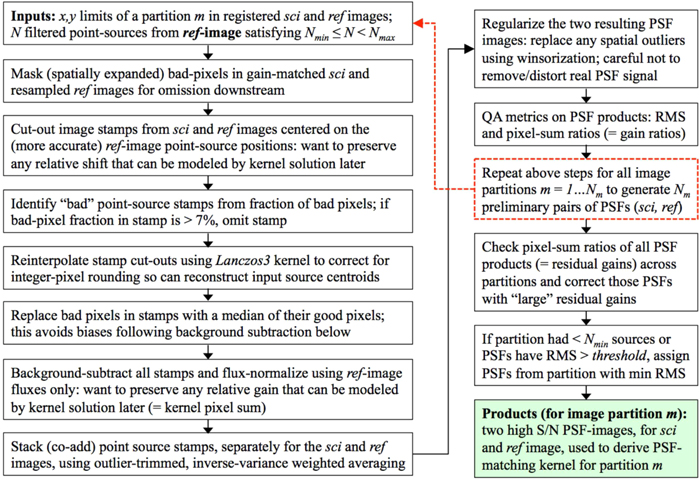
Figure 6. Processing flow for the creation and allocation of PSF image products for each common science and reference image partition. These are used to derive the spatially dependent PSF-matching kernel between the science and reference image. See Section 4.6 for details.
Download figure:
Standard image High-resolution imageFor a given image partition m, square stamps of linear size –psfsz (=25) pixels centered on the reference-image-based source centroids are cut from the (already registered) science and reference images. The reason for using the same (reference) position on both images is that we want to preserve any possible local astrometric shift between stamps of the same source from each image. This shift (if significant) will persist into the final respective PSF images and be subsequently captured by the kernel solution K(u, v). This will allow any local systematic shifts to be corrected following the application of K(u, v) to its respective image partition (Section 4.8). The point-source cutouts are then filtered to remove cases with large numbers of masked pixels. Each stamp is then interpolated into a new pixel grid so that the input (fractional-pixel) source centroids are made to fall close to their geometric centers, i.e., to correct for the truncation error when creating the initial cutouts using integer pixel coordinates. This registration step is important prior to stacking the point-source stamps. The stamps are then background-subtracted to ensure a zero-median background level outside an aperture with size specified by –apr. Pixel signals inside this aperture from only the reference image cutouts are then integrated and used to flux-normalize each matching science and reference image cutout of the same source. The reason is similar to that mentioned above for source positions—it preserves any possible residual in the relative gain that can later be modeled and removed by K(u, v).
If the debug switch was set, the point-source image cutouts can be individually written to FITS format with file suffixes _noconv_pm_stpn.fits and _toconv_pm_stpn.fits for the science and reference image respectively, where  is the partition identification index and
  is the source index therein.
The homogenized point-source cutouts for partition m are then separately stacked for the science and reference images. The first step involves using robust statistics to identify and mask outlying pixels in the pixel stacks. The stamps are combined using a weighted average where weights are the inverse of the pixel variances computed from the background in each stamp (outside an aperture with radius –apr). This results in two PSF images for partition m, one for the science and another for the reference image. The PSF images are further cleaned for possible pixel outliers using Winsorization (e.g., Kafadar 2003). Here, pixels that exceed some threshold (a multiple of the robust spatial rms above or below the background) are replaced with the threshold value. This replacement (when used with a high threshold) does not inadvertently distort the PSF shape. The input parameters and thresholds for the above steps are specified by the –rpickthres input string.
The source-cutout and stamp-stacking process is performed on all Nm partitions. This results in two preliminary (science and reference) PSF images per partition, assuming there were enough point sources therein (i.e., exceeding Nmin). If the debug switch was set, these can be written to FITS format with filename suffixes _noconv_pm_psfcoad.fits and _toconv_pm_psfcoad.fits for the science and reference image respectively, where  is the partition index. Accompanying pixel-depth maps showing the final number of stacked pixels are also generated with _psfcoad.fits replaced by _psfcoaddepth.fits in these filenames.
These PSFs are preliminary in the sense that there is no guarantee that all are of sufficient quality with good overall S/N across all partitions. For example, a partition could fall on a highly confused region, exhibit a complex background, or not have enough good quality point-sources. To account for this, we further regularize the PSFs for approximate consistency across all partitions. This includes replacing a bad PSF with a better quality one from a neighboring partition. A consequence of this replacement is that the selected PSFs (for a common science and reference partition) will no longer represent the true PSF shapes for that partition. This is a small loss since this replacement does not occur often, and when it does occur, the overall PSF variation is small enough that the impact to the PSF-matching is negligible when another partition's PSFs are used. These regularization steps are described in more detail below, with control parameters also specified by the –rpickthres input.
We first correct any PSF pairs with a large residual gain relative to all other PSF pairs from other partitions. The residual gain is estimated using the ratio of the sum of normalized PSF pixel values for the pair. Ratios that deviate by more than some threshold from the median pixel-sum ratio over all partitions have their respective PSF pixels rescaled to match the median ratio. This median ratio is typically unity due to the global gain-matching performed earlier (Section 4.2). Note that this "gain-homogenization" is only intended to correct PSF pairs with large outlying residuals in their relative gain. Next, we allocate the final PSF pairs to each partition by enuring that first, there were enough sources to make PSFs in the first place (i.e.,  ) and second, that the RSS of their robust spatial RMSs were below some threshold. If either of these conditions are not satisfied for a partition, we assign PSFs from that partition with the lowest RSS'd rms value. Each overlapping science and reference image partition is now associated with a high quality pair of PSFs, ready for the PSF-matching step. Figure 7 shows an example of the PSFs for two image partitions and the resulting matching kernels K(u, v) using the formalism in Section 4.7. As expected, the reference image PSFs will have a higher S/N and appear smoother since the references were initially created from a stack of science images.
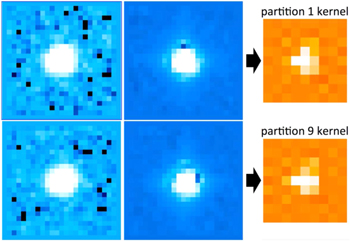
Figure 7. Example PSF image products for two separate image partitions: top row corresponds to a partition at the bottom left of a CCD image and bottom row is for a partition at top right of the same image. From left to right: PSF for science image, PSF for reference image, and the resulting PSF matching kernel derived using the method in Section 4.7. Pixel sizes are the same throughout. The kernel images are enlarged for clarity.
Download figure:
Standard image High-resolution image4.7. Derivation of PSF-matching Kernel
Given high S/N representations of the science and reference-image PSFs for a spatial partition, with PSF pixel values Iij and Rij respectively at common coordinates i, j, we outline below the method used to obtain an optimal solution for the convolution kernel K(u, v) and differential background dB in Equation (13). Following previous approaches, these can be derived by minimizing a weighted sum of the squared residuals between a model and some new image (here the science image PSF); for example, using the objective function
where  are prior pixel uncertainties in the Iij that may include some scaled contribution from Rij (see below). Equivalently, Equation (14) can be recast in vector-matrix notation:

where  is the full error-covariance matrix to account for possible correlated errors between the input pixels, and M is the model-image with elements:

Strictly speaking, the objective function  can only be compared to a true χ2 distribution with degrees-of-freedom Ndof for the purpose of validating model solutions using probabilistic inference if the input data errors are normally distributed; i.e.,
  . These errors can be interdependent (and if so, need to be captured by Ωcov), but they do need to be identically distributed for χ2-validation purposes. The null hypothesis is that the model (Equation (16)) "generated" the Iij. Furthermore, for linear parameterizations of K(u, v) (see below), the minimization of
  reduces to a generalized linear least-squares problem with a solution that is unique and optimal in the maximum-likelihood sense for normally distributed errors.
Another important consideration is that the input errors  are heteroskedastic, i.e., they are not identically distributed with constant variance over the input pixels i, j. This is because we are exclusively fitting point-source data where Poisson noise dominates. The noise-variance will have a spatial dependence following the shape of the PSF profile (Iij). Even though this dependence can be accounted for by using prior weights derived from the pixel uncertainties (
 or
or  ) that implicitly include Poisson-noise, their direct use in
  will lead to biased estimates for K(u, v) and dB. This was explored in a different context by Mighell (1999). A number of complex variance-stabilizing methods exist to ensure unbiased estimates. For simplicity, we omit the use of prior weights when estimating K(u, v) and dB. Our solution will still be optimal in the least-squares sense and will also be close to the maximum-likelihood solution for normally distributed errors in general. Even though the exclusion of weighting in Equation (14) prohibits the use of goodness-of-fit tests in an absolute (probabilistic) sense, relative changes in the global
  can be used to validate the performance of different kernel solutions when applied to full images (see Section 4.8.2). For completeness, we continue to carry the σij term (as represented in Equation (14)) in our derivations below. In the end, our estimates are really solutions to an ordinary linear least-squares (OLS) problem.
Our construction in Equations (13) and (14) assumes that the image containing the narrower PSF is the one that should be convolved. However, there is no guarantee that this image is always the reference PSF (Rij) and hence without loss of generality, Iij and Rij can be interchanged. It is therefore important to predefine the convolution direction. This can be specified by the–conv input string. The choices are sci, ref, or auto. The sci and ref options always force the science (Iij) or reference (Rij) image pixels to be convolved respectively. The auto option allows an automatic selection of the image to convolve and is our current operating mode. This selection is based on comparing global-image measures of the FWHM values of filtered stars from the science and reference images. The FWHM values are from 2D Gaussian fits performed by SExtractor. These values are medianed to yield two measures: FWHMsci and FWHMref. The automatic selection is based on the value of the relative difference

Currently if  , the science image is selected for convolution, otherwise the reference image is selected, i.e., as depicted in the estimation equations above. The threshold for δ was tuned by examining distributions in FWHMsci and FWHMref from many images and setting a conservative value to allow for uncertainty in the median FWHM estimates. In other words, the fuzzy interval
  implies the overall sci and ref PSF FWHM measures are consistent within measurement error. Note that the FWHM measure is assumed to be a good proxy for PSF shape in general, at least to first order for the purpose of defining a convolution direction. When the PSF FWHMs are consistent, no useful information is expected in the kernel solution, i.e., aside from noise and perhaps variations incurred by higher-order PSF-shape differences. The kernel then effectively becomes a single spike (i.e., a δ-function) where in principle, no PSF-matching would be required.
Usually (for ≳85% of science image exposures encountered), the reference images are those selected for convolution since by design, these were constructed from archived science images with moderately better seeing than average, in addition to being weighted by their inverse-seeing (Section 3.3). However, for cases where the science image (Iij) is selected for convolution, the roles of Iij and Rij are interchanged in Equations (14) and (16) so that Iij convolved with K(u, v) becomes the model-image fitted to the data, Rij. This complicates the error and weighting structure if a true χ2 objective function (based on Equation (14)) were to be used for estimation since the model would be noisier than the data being fitted. This is another reason for omitting the use of prior weights in the objective function and treating it as a simple OLS problem. The application of K(u, v) to the noisier Iij image also causes a larger fraction of the noise to be correlated in the final difference image. This is further discussed in Section 4.8.
As mentioned above, linear parameterizations for K(u, v) are the simplest to solve from a computational standpoint, for example, by expanding K(u, v) as a linear combination of n basis functions:
and solving for the n coefficients ai. A traditional choice for the Ki(u, v) are Gaussians of different width, each modified by a 2D shape-morphing polynomial. The ai are further expanded into another polynomial in x, y to model possible dependencies over the focal plane. This is the classic PSF-matching algorithm of Alard & Lupton (1998) and Alard (2000), and extended by Yuan & Akerlof (2008). This algorithm has been successfully used by several time-domain surveys, e.g., OGLE (Wyrzykowski et al. 2014), La Silla-QUEST (Hadjiyska et al. 2012), Pan-STARRS (Kaiser et al. 2010) and the SDSS-II Supernova Survey (Sako et al. 2008). Initially, we extensively validated this method for PTF (at IPAC, Caltech) as implemented in the HOTPANTS14 and DIAPL utilities (Woźniak 2000). A major limitation was the specification of a number of fixed configuration parameters. These parameters are not fitted, i.e., the Gaussian widths (at least four were needed) and the polynomial orders (six more parameters). The overall performance was sensitive to the precise choice of these parameters. Furthermore, the basis functions were not complex or flexible enough to model the bulk of the data encountered in the survey, under a continuum of atmospheric conditions and unforeseen instrumental behaviors. Despite attempts to constrain the basis function constants using a priori information in a dynamic manner (e.g., as prescribed by Israel et al. 2007), a generic-enough representation for K(u, v) under this framework that kept the false-positive rate among transient candidates appreciably low and at a manageable level eluded us.
A more flexible "shape free" basis representation for K(u, v) was proposed by Bramich (2008). Here the kernel is discretized into L × M pixels and each pixel value therein, Klm, is treated as a free parameter in the OLS fitting problem. This free form basis is also referred to as the delta function representation where the kernel can be expressed as a 2D array of delta functions:

A kernel size of 9 × 9 pixels (input parameter–kersz) then has 81 orthonormal basis functions when expanded as a linear combination according to Equation (18). For comparison, the best Gaussian-basis model mentioned above has 252 free parameters for effectively the same amount of input data in the estimation process. Apart from the kernel image size and threshold parameters used to creating the regularized PSF-inputs (Section 4.6), there are no shape-based tuning parameters for the delta-function representation. For this reason, it can accomodate more generic shapes, as well as capture offsets in the astrometry on scales used to construct the input PSF data Iij and Rij, coming from effectively a Nx × Ny image partition. As we shall discuss, this unconstrained specification is both good and bad.
With this representation, the model image (Equation (16)) can be written in terms of the unknown coefficients Klm as follows:

The objective function to minimize (the equivalent of Equation (14)) then becomes
The optimal values of Klm and dB are those that minimize  , i.e., where the partial derivaties of
  with respect to each parameter are all zero:
These are evaluated at the specific parameter values indexed by  for Klm and dBo to yield two general relations:
and
respectively. The kernel pixel indices in Equations (23) and (24) have the ranges
where  corresponds to the center pixel of the kernel with dimensions L × M pixels and p is a one-dimensional index: p = 1, 2, 3, ..., LM. For a given lo, mo,

Equations (23) and (24) lead to a simultaneous system of LM + 1 equations in LM + 1 unknowns that can be written in the vector-matrix form:

where X is a vector containing the LM kernel-pixel unknowns Kp (=Klm) and differential background estimate dBo.
Equation (27) can be inverted using standard techniques, and at first, X was estimated directly using a LU-decomposition of A. However, in accord with previous analyses (e.g., Becker et al. 2012), the unconstrained nature of a pure delta-function representation can make the Klm solutions very sensitive to noise and contamination from non-PSF related signal in the inputs Iij and Rij. The model-fit is therefore subject to over-fitting. This is the so-called bias versus variance tradeoff where one is after a solution that is expressive enough to avoid biases, but not so complex as to introduce excessive variance when the solutions are later applied to match the PSFs in an entire input image or partition. In the end, one is after the true PSF-matching kernel for the two images. Despite our attempts to mitigate noise in the input PSF co-add stamps (Iij and Rij; Section 4.6), noise is inevitable. One way to avoid overfitting and still maintain optimality is to invoke regularization in the estimation process.
4.7.1. The Regularized PiCK Method
Becker et al. (2012) implemented a regularized version of the delta-function kernel model by introducing a tunable smoothing constraint in the χ2 objective function. This function is proportional to the second spatial derivative in the input pixels and is intended to penalize fits that are too irregular as a result of high-frequency noise. This regularization method was explored and validated in detail by Bramich et al. (2016) from the aspect of maximizing photometric accuracy in final difference images. This extension is attractive, but it did not become known to us until after we had implemented an alternative regularized version of the delta-function model (see below). This worked very well on PTF image data. We will refer to this method as the Pixelated Convolution Kernel method (or PiCK for short).
Instead of imposing a regularizing constraint on the objective function as in Becker et al. (2012), our approach involves regularizing the coefficient matrix A in Equation (27). We perform a spectral decomposition, also known as an eigendecomposition of A:

where V is an orthogonal matrix ( ) and W is a diagonal matrix:

with eigenvalues  . The corresponding linearly independent eigenvectors of A reside in the columns of V. Given A is a real symmetric matrix, such a decomposition can always be found. This decomposition allows us to examine the basis vectors that will contribute to the kernel solution. The least-important eigenvectors of A are those associated with input noise and can be identified by their relatively small eigenvalues, below some threshold. These can then be "zeroed-out." For example, the inverse of A can then be written

where

for all  . For values wi = 0 (within machine precision), the
  are replaced by zero in
  . This special replacement corresponds to the classic Singular Value Decomposition (SVD) method for handling singular (ill-conditioned) matrices. The inverse defined by Equation (30) then becomes the pseudo-inverse of A. This approximation is better conditioned for obtaining a solution to the matrix equation in (27).
The essence of the PiCK method is to make this SVD-like replacement more generic and less restrictive on the specific wi to replace. The goal is to also make A more regularized against noisy input data (including singular cases) by finding the largest eigenvalue wk such that  for some threshold T (see below). For all
  , we reset
  in W−1 and then proceed to obtain a solution. Following the decomposition in (30), the solution vector X in Equation (27) can be written
In this form, it can be seen that the noisiest (least-relevant) eigenvectors Vi according to  will not significantly contribute to X. Therefore, they can be eliminated by forcing
  . These eigenvectors can be also identified by their relatively small dot-products with the B vector,
  , as shown in Figure 8.

Figure 8. Relative eigenvalue strength (crosses) and eigenvector magnitude (circles) vs. eigenvector index i. Increasing i corresponds to progressively higher spatial frequencies, eventually approaching the pixel noise. Horizontal dashed lines correspond to dynamically derived truncation thresholds; see Section 4.7.1. Results are shown for two kernel solutions derived for image partitions with two different source densities, left: moderate to low-density typical of high galactic latitudes; right: a density that is ∼80× higher.
Download figure:
Standard image High-resolution imageThe threshold T is dynamically derived on a per image-partition basis, i.e., where an inversion of Equation (27) via (30) is performed. This uses the following semi-empirical criterion:
where the second argument corresponds to the low-tail percentile of the max-normalized wi distribution. The values in Equation (33) were tuned by examining the eigendecompositions of A using iPTF image data acquired across different environments, from low source-density to densities approaching those in the galactic plane. A range of T values were then tested by exploring the impact of the corresponding regularized solutions on the overall fit χ2 (Equation (21)). Examples of these eigendecompositions are shown in Figure 8. The criterion in Equation (33) corresponds to approximately an inflexion point in the relative eigenvalue size. This choice is also conservative in the sense that the amount of legitimate high-frequency information thrown away (not associated with noise) is expected to be insignificant as determined by the change in χ2 with and without regularization (T = 0). I.e., we ensure that  , where ν is the effective number of degrees of freedom. In the current setup for iPTF,
The regularization threshold T is also dependent on the size of the kernel assumed (=L × M free parameters to solve) since this determines the relative fraction of noise contributing to the Klm estimates. The kernel image size was tuned beforehand to be small enough to avoid introducing too many free parameters that would result in overfitting on noisy backgrounds in the PSF stamps, but large enough to accomodate the range of seeing (point-source profile widths) encountered. This ensures both unbiased kernel solutions and minimal variance following their application, i.e., a compromise in the bias versus variance tradeoff mentioned above.
When a PSF-matching kernel image with estimates Klm is available, a measure of the relative residual gain between the science and reference image pixels for a specific image partition (from which Iij and Rij were extracted) is given by the sum

The Ksum values (across all image partitions) can be used to assess the accuracy of the global relative gain correction computed upstream (Section 4.2.1). More importantly, they provide local estimates of any residual photometric gain where if significant, can be used to refine the gain factor at the image partition level prior to differencing (see Section 4.8). Ksum also provides a diagnostic to assess the quality of the kernel solution. For example, an image partition with a Ksum that significantly deviates from unity compared to that of its neighboring partitions could indicate a problem in the estimation process, perhaps triggered by bad or low-quality input PSFs. For details, see the discussion on quality assurance in Section 4.8.2.
To summarize, we have extended the free form delta-function model representation to derive PSF-matching kernels by performing a simple regularization of the matrix system used for the least-squares solution. This uses an eigendecomposition to retain the most significant basis vectors within a statistically validated threshold. We have coined this the PiCK method. Figure 9 shows examples of input images, kernels, and the resulting difference images for a relatively dense field with and without regularization included. The relative change in χ2 (Equation (21)) going from the unregularized to regularized solution for the entire image shown in Figure 9 is ≈−3.5%. The PiCK method leads to smoother PSF-matching kernels and hence difference images in general. It is also robust against contamination in the input PSFs (Iij and Rij), for example when constructed from high source-density regions.
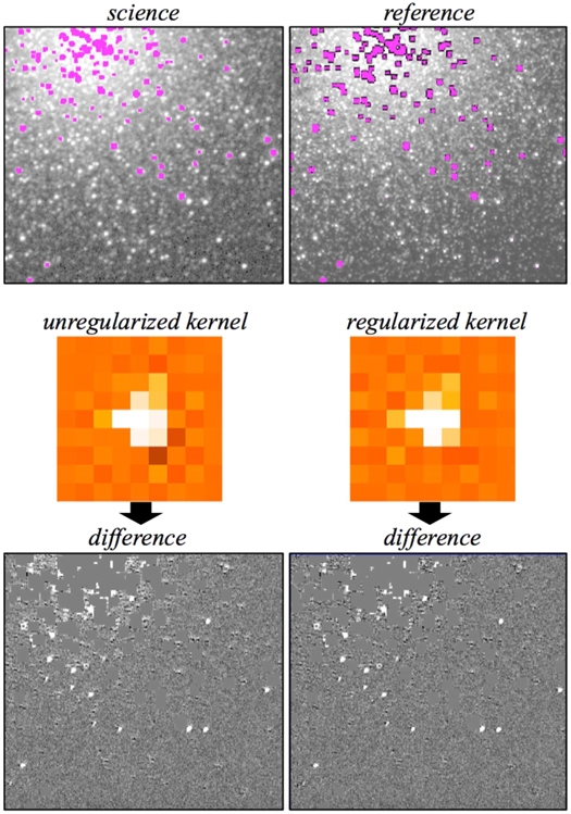
Figure 9. Top left and right: zoomed-in region on a preprocessed science and resampled reference image respectively containing a portion of the M13 Globular Cluster and measuring ≃5' on a side. The magenta regions are saturated pixels. Middle left and right: PSF-matching kernels based on no regularization (from a naïve inversion of Equation (27)) and with regularization respectively (Section 4.7.1). These are enlarged for clarity. Bottom left and right: difference images resulting from "science minus kernel-convolved reference" for the unregularized and regularized kernels respectively. Saturated pixel regions were reset to zero in the difference images. These were also spatially expanded from their original size (top images) due to the convolution process. The bright source-like residuals in the difference images are on the locations of known RR-Lyrae variable stars. For an animation of products for the entire CCD across multiple epochs, see http://web.ipac.caltech.edu/staff/fmasci/home/idemovies/d4335ccd8f2movie.html.
Download figure:
Standard image High-resolution image4.8. Kernel Application and Difference Image Products
The PSF-matching convolution kernel is first normalized to unity to yield

where Ksum was defined by Equation (35).  is then convolved with the specific image partition that was initially selected for convolution using the method in Section 4.7, i.e., defining the convolution direction. The reason for decoupling Ksum (the local relative gain factor) from the raw kernel Klm is so that any residual gain correction can be refactored and applied as a multiplicative correction on the science image pixels only, and not the resampled reference image, regardless of the convolution direction. This is consistent with our modus operandi in PTFIDE: all corrections are applied to the science image pixels, in order to match the photometrically and astrometrically calibrated reference image as best as possible.
If the reference image was selected for convolution, the difference image pixel values for an image partition from which the kernel and differential background estimates were derived can be written:
If the science image was selected for convolution, the difference image pixel values for the image partition can be written:
Two difference images per science, reference image pair are generated, a positive (sci—ref) and negative (ref—sci) difference image. As described in Section 3.4, this is to enable the detection of transients and variables that happen to be below the reference-image baseline level at any observation epoch. The positive and negative difference images are written to FITS formatted files with filename suffixes _pmtchscimref.fits and _pmtchrefmsci.fits respectively. If the debug switch was set, ancillary products representing the different components of Equations (37) or (38) prior to differencing can also be generated (see Table 4). These are the final science image, convolved or not with Ksum and dBo applied: _scibefdiff.fits, and the convolved counterpart: either  or
or  : _pmtchconvref.fits or _pmtchconvsci.fits respectively.
The science and reference image bad-pixel masks generated upstream (Section 4.1) include the effects of convolution where bad pixel regions are expanded accordingly. These are combined to produce a final effective bad-pixel mask for both the positive and negative difference images. If the debug switch was set, this can also be written to FITS format with filename suffix _pmtchdiffmsk.fits. Furthermore, all bad pixels in the difference images are tagged with value −999,999.
An image of the 1-σ uncertainties corresponding to the Dij images (Equations (37) or (38)) is also generated. These uncertainties are estimated by RSS'ing the input uncertainties for the science and reference images (Equations (11) and (12) respectively in Section 4.5) with a correction for correlated-noise:

The correlated-noise correction factor Fc accounts for the diminution in the pixel rms noise (lost to covariance) due to the convolution process. Recall that this convolution may have been performed on either the science or reference image (see above). Fc is approximated as the ratio of the robust pixel rms in the actual difference image to the RSS'd background RMSs in the science and reference images prior to any convolution:
The background variances in the denominator of Equation (40) are the same estimates used in Equations (11) and (12) of Section 4.5. The presence of correlated-noise in the difference image will underestimate the photometric uncertainties of extracted sources therefrom if not properly accounted for on the spatial scales of interest (i.e., the spatial-extent on which the photometry is performed). Note that Fc does not represent any correction at the source level. Its purpose is to capture any modification to the input uncertainties (σsci and σref) due to smoothing from the PSF-matching process. The source level correction is computed and applied during the source extraction step (see Section 4.9.2).
4.8.1. Photometric Zeropoint Quality Check
Following application of the spatially dependent convolution kernels and associated gain-corrections (Ksum) to the science image pixels (Equations (37) and (38)), we compute a new photometric zeropoint for the adjusted science image. This ZP will also be applicable to the difference images generated therefrom. It provides a sanity check on the global-image ZPSCI value computed upstream using the input absolutely calibrated reference image photometry (see Section 4.2.2). As mentioned, ZPSCI enables a more accurate absolute calibration of either PSF-fit or big-aperture photometry.
The new ZP is only computed if the–phtcaldif switch was specified on input. If so, it is written as the ZPDIF keyword with accompanying rms ZPDIFRMS to the FITS headers of both the positive and negative difference images. The computation uses exactly the same methodology as outlined in Section 4.2.2. If the debug switch was set, a catalog of the reference-to-science image matches used to compute ZPDIF is generated with suffix _sx_scibefdiff.tbl. When the PSF-matching and additional gain-refinement steps perform as intended, ZPDIF is generally consistent with ZPSCI, within random measurement error. Large deviations in Δ ZP = ZPSCI − ZPDIF usually imply a problem with either the PSF-matching kernel(s), the input astrometry, or its later refinement since astrometric accuracy will indirectly affect the source matching step used to estimate the ZPs. Δ ZP therefore provides a powerful quality assurance metric.
4.8.2. Difference-image Quality Assurance Metrics
Metrics and diagnostics for a difference image product are shown in Table 6. These encompass information on photometric zeropoints; pixel statistics before and after PSF-matching; properties of the PSF-matching kernels; statistics on the input science and reference images; global image FWHM values; and the number of candidates extracted (Section 4.9). These metrics are used to support later machine-learned vetting (Section 6).
In PTFIDE processing, two checks are performed to assess the quality of the difference image: (i) "atrocious" and unusable for extracting candidates, and (ii) simply "bad" and warranting visual examination before use. PTFIDE does not extract candidates if (i) is satisfied, but does proceed to extract candidates if (ii) is satisfied. The indicator flag for either condition is the status flag in Table 6 [=0 (bad) or 1 (good)]. Even though candidates are extracted under (ii) during processing, these are not loaded into the database (Section 5). The rationale is that bad subtractions will lead to thousands of spurious candidates and strain both database loading as well as machine-learned vetting downstream. The conditions for (i) and (ii) are determined using one-dimensional cuts on a number of metrics from Table 6 as follows.
First, a difference image is flagged atrocious if the following criteria are satisfied:
where in terms of the metrics listed in Table 6,
and the seven thresholds (thresai) are specified by the–uglydiff input string with defaults defined in Table 2.
If the difference image is not labelled atrocious according to the criteria in (41), it is subject to the less-severe criteria below. These are applied after transient candidates are extracted. The metrics used here are therefore a subset of those from above (but with lower "badness" thresholds) and others related to the number and properties of candidates extracted. See Table 6 for definitions.
The 11 thresholds (thresbi) are specified by the–baddiff input string with defaults defined in Table 2. If the criteria in (43)8 9 are satisfied, status = 0 is assigned to indicate a possibly bad difference. This flag is propagated to the subtractions table of the transients database (Section 5).
Table 5 summarizes the percentages of atrocious, bad, and good difference images obtained from real-time processing for two sky regions spanning different galactic latitudes and longitudes. These regions sample the extremes in source-density: near the galactic center and bulge, and high galactic latitudes. These were covered by iPTF from 2015 August to 2016 January. The high fraction of failures near the galactic center (or bulge) can be attributed to adverse effects from high source confusion on the processing steps prior to differencing, for example, astrometric calibration, and/or gain and PSF-matching. All these steps depend on source-matching of some kind between the science and reference images, and is severely challenged in regions of high source density. For examples of bad or unusable difference images and their causes, see Section 6.2.
Table 5. Difference Image Quality Statistics
| Quality |
 
|
 
|
|---|---|---|
| (1824 diff. images) | (7629 diff. images) | |
| atrociousa | 25.0% | 0.42% |
| badb | 34.5% | 11.18% |
| goodc | 40.5% | 88.40% |
Notes.
aFlagged according to the criteria in (41). bFlagged according to the criteria in (43). cSatisfy neither (41) or (43).Download table as: ASCIITypeset image
If the debug switch was set, an image of the locally smoothed pixel chi-square is generated for both positive and negative difference images. This is analogous to a reduced χ2 and is defined as
where the angled brackets denote boxcar averaging over pixels i, j that fall within 8 × 8 pixel bins over the difference image. The image generated from Equation (44) is written to a FITS formatted file with suffix _pmtchdiffchisq.fits. Large values in  (significantly above unity) may indicate residuals from imperfect instrumental calibrations, underestimated pixel uncertainties, or the presence of real transient sources. Small values (
 ) will imply that the pixel uncertainties are overestimated.
4.9. Candidate Transient Detection and Photometry
The detection and photometry of transient candidates on both the positive and negative difference images is performed using an automated implementation of the DAOPhot tool (Stetson 1987, 2000). This includes the subsidiary program Allstar which performs PSF-fit photometry on the detections found by DAOPhot. The primary output photometry for characterizing transient candidates is PSF-fitting. Fixed concentric aperture photometry is also generated as a diagnostic. The benefits of PSF-fit photometry cannot be stressed enough, at least for detecting transient events. For example, this provides better photometric accuracy to faint fluxes; the ability to de-blend confused sources; and simple metrics to distinguish point (PSF-like) sources from artifacts. These metrics can be used to maximize the reliability of candidates.
Perl routines were written to automate all decision-related and processing steps in DAOPhot. These steps would have been done interactively in classic DAOPhot. This includes all file I/O, parameter handling, checking of outputs, and quality assurance. The steps are summarized below.
4.9.1. Point Source Detection
DAOPhot first detects sources for input into either the PSF-determination step or final PSF-fitting step using a matched filter via its find algorithm. The filter is constructed from a Gaussian with a proxy for the image FWHM computed upstream using SExtractor on the science image. This Gaussian is convolved with the image in question to construct the point-source matched filter, i.e., an internal product that is optimized for point-source detection. This assumes that the PSF is approximately spatially uniform over the image, and for the purpose of detection, the penalty in detection S/N by not using the precise spatially varying PSF is negligible. This image is then background-subtracted using local estimates of the background. The pixel-uncertainty product from Equation (39), which effectively includes contributions from detector read-noise, background, and Poisson noise at the location of sources, is internally readjusted to account for the matched filtering. The ratio of the match-filtered, background-subtracted image and its corresponding uncertainty image is then thresholded. Either the–tdetpsf or–tdetdao S/N parameter threshold is used depending if PSF-determination or final dectection is desired respectively. If the debug switch was set, the detection tables from these steps are written to files with extension .coo (see Table 4 for filenames).
4.9.2. PSF Determination, PSF-fitting and Aperture Photometry
PSF generation and PSF-fit photometry (or source extraction of any form) are only attempted if the input difference image was determined to be of sufficient quality according to a number of quality metrics (see Section 4.8.2). If not, PTFIDE processing terminates gracefully after the image differencing step. Furthermore, PSF-fit photometry can be intentionally turned off by omitting the–psffit switch.
The base parameters specific to DAOPhot and Allstar reside in configuration files specified by–cfgdao and–cfgpht, with some of the more important (threshold-like) parameters therein overridden by the command-line inputs: –tmaxpsf, –tdetpsf, and –tmaxdao. Also, some parameters are computed dynamically within ptfide.pl and override those from both the input files and command-line. These parameters are those that depend on the image noise, usable pixel range, and image FWHM: RE, LO, HI, FW, PS, FI, and nested aperture radii Ai where i = 1...6. The parameters that depend on the input FWHM (FW) are the linear-half-size of the PSF image stamp, PS (for PSF-creation only); the PSF-fitting radius, FI; and the aperture radii Ai, all in units of pixels. Respectively, these parameters are adjusted according to
where i = 1...6, and min, max, int denote the minimum, maximum, and integer part of the argument respectively.
When ptfide.pl is run in PSF-fit photometry mode (with the –psffit switch), only one aperture measurement corresponding to a single fixed aperture is written to the primary output tables: file suffixes _pmtchscimrefpsffit.tbl and _pmtchrefmscipsffit.tbl for the positive and negative difference images respectively. This is the aperture number i corresponding to the user-specified parameter –apnum (currently = 3). If however, the –apphot switch was also specified, all nested aperture measurements (i = 1...6) are written to separate tables with file suffixes _pmtchscimrefapphot.tbl and _pmtchrefmsciapphot.tbl. These products are not currently generated in production. It is important to note that the aperture measurements are not curve-of-growth corrected to account for the variable seeing. They only serve as diagnostics (or source features; Table 7) to support machine-learned vetting (Section 6).
The PSF used for PSF-fitting is estimated automatically using utilities within DAOPhot and Allstar. Its shape over a CCD image is modeled as a linear function in x, y. This dependence is sufficient to catch spatial variations in the PSF and avoids introducing too many free parameters. The PSF is always estimated from the resampled and possibly convolved reference image (following PSF-matching). This is because the reference image (convolved or not) is expected to have a higher S/N than the science image. In the end, we want to estimate the PSF on an image whose point-source profiles match those in the difference image (either positive or negative). In theory, given that the only operations performed on the input images prior to differencing are gain, background and PSF-matching, and given that differencing is a linear operation, either the science or reference image would have sufficed for PSF estimation.
For iPTF, no more than the brightest 200 point sources with magnitudes  are automatically selected per CCD image to estimate an initial spatially varying PSF. This is refined in a second iteration by subtracting neighboring sources (in the wings) from the initially chosen PSF stars and then re-estimating the PSF. This second iteration can be rather slow if there are many neighbors since it involves PSF-fitting to obtain the fluxes and positions of the neighbors to subtract. To speed up the process, we regulate the number of neighbors to consider by only subtracting the brightest 1000 neighbors to all the initially PSF-picked stars. Therefore, given a random distribution of sources and
  sources picked for PSF generation, ≳5 (brightest) sources on average will be subtracted prior to refinement of the PSF in the second iteration. This makes the PSF estimation relatively fast and robust, and there are always enough stars in an image to yield a reasonably accurate PSF model.
The PSF model is stored in the default DAOPhot format, with output file suffix _pmtchconvrefdao.psf if the reference image was convolved, otherwise _resamprefdao.psf if the science image was convolved. This file consists of a look-up table of corrections to a best-fitting Gaussian basis model over the image. Other basis functions are available, but we found a Gaussian works reasonably well for PTF data (in terms of photometric accuracy). This basis representation also has the least number of free parameters. If the debug switch was set, the DAOPhot-formatted PSF file is converted to a FITS image of 16 × 32 PSF-stamps for visualization (output file suffix _pmtchconvrefdaopsf.fits). Other ancillary files, e.g., the list of PSF-picked stars, their neighbors, and DS9 region files are also generated (see Table 4).
Following PSF estimation, sources are detected on the positive and negative difference images above a specific threshold as described in Section 4.9.1. PSF-fit photometry is then performed using Allstar. This program estimates seven quantities per input detection: flux; flux uncertainty (to be rescaled later, see below); refined image x, y position; uncertainties in x, y; and two metrics from the fit: chi, and sharp (see below). We do not iteratively subtract the PSF to uncover new sources that were missed in the first detection pass, e.g., because they were hidden in the wings of brighter sources. This is commonly done for crowded fields. Given we are extracting sources from difference images, source-crowding (or rather, blending of transient candidates) is largely absent, even in areas of high source density. One can argue however for cases where instrumental residuals could blend with real transient sources. This is also rare, but nonetheless the components of a blend only need to be detected in the first place so that simultaneous PSF-fitting can yield fluxes and other metrics for further examination downstream.
The PSF-fit fluxes are converted to absolute calibrated magnitudes using the ZPSCI image zeropoint computed upstream (Section 4.2.2). This places the photometry on the PTF filter system (Ofek et al. 2012). Note that the supposedly refined ZPDIF value (Section 4.8.1) is not used since analyses have shown that it exhibits a greater variance than ZPSCI. This arises from systematics in the PSF-matching and relative gain-matching process. The source x, y positions are converted to R.A., Decl. using the difference image WCS (inherited and refined from the reference image WCS). This information is written to the transient-candidate extraction tables (one for each difference image; see above). DS9 region files also accompany these tables (see Table 3 for filenames).
4.9.3. Correcting Uncertainties for Correlated Noise
Another detail is correcting the flux uncertiainties from PSF-fitting for correlated pixel-noise in the difference image. As discussed in Sections 4.5 and 4.8, correlated noise arises from the reference-image construction process (interpolation and resampling), but the more dominant effect is from convolution by the PSF-matching kernel, where either the science or reference image may have been convolved. Given that the reference image has a higher S/N in general, and that this is the image that is usually convolved (by design), the fraction of the pixel noise that is correlated in a difference image is likely to be small. For example, if the reference image is made from a stack of Nf science images all with similar pixel noise-variances, the fractional contribution to the difference image pixel-noise from the (convolved) reference would be  . If the science image were convolved however, the fractional contribution would be greater, i.e.,
 ![$\simeq {(1+[1/{N}_{f}])}^{-0.5}$](https://content.cld.iop.org/journals/1538-3873/129/971/014002/revision1/paspaa443cieqn137.gif) , approaching 100% if Nf is large.
, approaching 100% if Nf is large.
We use a simple method to correct the source-flux uncertainties from PSF-fit photometry before writing them to the photometry tables. The flux uncertainties from Allstar are estimated using some combination of the difference image pixel uncertainties (Equation (39)) within the effective fitting area of the PSF. Following convolution (smoothing) of the one of the images, these will underestimate the true source-flux uncertainty. The true uncertainty contributed by the convolved image can be recovered by scaling its pixel uncertainties by the effective number of noise pixels17 defining the convolution kernel:
where  are the unit-normalized pixel values of the kernel image (Equation (36)). Nk effectively represents the correlation length (or in this case the correlation area) in pixels. Therefore, we seek a correction factor C for scaling the difference image source flux variance which can also be written in terms of its science and reference image contributions, after convolution by
  :
:

where we assume (for illustration) that the reference image was convolved. If the science image was convolved, Nk would be multiplying the science image variance term. Since all the flux-variance terms in Equation (47) are some weighted combination (or effectively an RSS) of the pixel noise variances, in the limit of background-dominated noise, the correction factor can be estimated from
where the variances now denote robust estimates of the background pixel rms in the science, [convolved] reference, and difference images. These quantities are estimated within respective image partitions, i.e., the same partitions used to compute the kernel images (and hence Nk). This construction was verified using Monte Carlo simulations (see footnote 17).
4.9.4. Coarse Filtering of Raw Candidates
The raw candidates initially extracted from the difference images as described in Section 4.9.2 undergo loose filtering prior to writing them to the transient-candidate tables (file suffixes _pmtchscimrefpsffit.tbl and _pmtchrefmscipsffit.tbl for positive and negative difference images respectively). The intent is to catch the most deviant non-PSF-like residuals from the difference images and remove them. This somewhat relieves traffic on database loads (Section 5) and the machined-learned vetting step (Section 6) which also heavily relies on interactions with the database.
This simple filtering can result in reductions of up to a factor of five in the number of raw transient candidates initially detected from the point-source match-filtered image down to S/N ≃ 3.5 (–tdetdao input threshold; Table 2). It is worth mentioning that this relatively low initial detection threshold is to ensure completeness prior to further filtering and analysis downstream, including photometric S/N. The filtering applied to the raw detected candidates is 

 , where the thresholds on the right are currently 8, 4, and 4 respectively (from Table 2).
All these parameters are source-based metrics from PSF-fitting and are defined as follows: chi—the ratio of the rms in PSF-fit residuals to that expected using prior pixel uncertainties; sharp—effectively the difference between the squared FWHM of the source light profile (from a 2D Gaussian fit) and that expected from the PSF template model derived for the image, i.e.,  and snrpsf—the photometric signal-to-noise ratio using the PSF-fitted flux and uncertainty. Relatively large values of chi and/or
  indicate deviations from the nominal PSF template estimated upstream for the difference image (Section 4.9.2). The optimum values of chi and sharp are 1 and 0 respectively. For example, a cosmic-ray spike would yield
  and an extended source
  , as well as
  for both these cases. The number of candidates that satisfy initial filtering using chi, sharp, and snrpsf are recorded as ncandfilt in the QA output table (Table 6).
Table 6. Difference Image-based Quality Assurance Metrics from PTFIDE
| Metrica | Description |
|---|---|
| zpmaginpsci | Photometric zeropoint (ZP) estimate of science image before rescaling to reference [mag] |
| zpmaginpsciunc | 1-σ uncertainty in zpmaginpsci [mag] |
| zpmagcormed | Median ZP correction offset to zpmaginpsci over all partitioned convolution kernel sums [mag] |
| zpmagcormin | Min. ZP correction offset to zpmaginpsci over all partitioned convolution kernel sums [mag] |
| zpmagcormax | Max. ZP correction offset to zpmaginpsci over all partitioned convolution kernel sums [mag] |
| zpmaginpscicor | Refined photometric zeropoint (ZP) of science image following application of kernel sums: "zpmaginpsci + zpmagcormed" [mag] |
| zpfacinpsci | Photometric scale factor applied to science image to match reference image ZP |
| zpfacinpsciunc | 1-σ uncertainty in zpfacinpsci |
| zpref | Photometric zeropoint (ZP) of input reference image [mag] |
| nmatch | Number of sources matched within 3.0 pixels between science and reference images to support initial gain-matching and astrometric refinement |
| fluxrat | Median flux ratio of matched sources prior to global gain-matching: fluxsci/fluxref |
| pctfluxrat | 5th–95th percentile range in 'fluxrat' values of matched sources |
| deltax | Median positional difference along X-axis using matched sources: Xref − Xsci [pixels] |
| sigdeltax | 1-σ uncertainty in deltax [pixels] |
| pctdeltax | 5th–95th percentile range in deltax values across matched sources [pixels] |
| deltay | Median positional difference along Y-axis using matched sources: Yref − Ysci [pixels] |
| sigdeltay | 1-σ uncertainty in deltay [pixels] |
| pctdeltay | 5th–95th percentile range in deltay values across matched sources [pixels] |
| medksum | Median pixel-sum of all image-partitioned raw convolution kernel sums |
| minksum | Minimum pixel-sum of all image-partitioned raw convolution kernel sums |
| maxksum | Maximum pixel-sum of all image-partitioned raw convolution kernel sums |
| medkdb | Median differential background over all image-partitioned raw convolution kernels [DN] |
| minkdb | Minimum differential background over all image-partitioned raw convolution kernels [DN] |
| maxkdb | Maximum differential background over all image-partitioned raw convolution kernels [DN] |
| medkpr | Median 5th–95th percentile pixel range of all image-partitioned raw convolution kernels |
| minkpr | Minimum 5th–95th percentile pixel range of all image-partitioned raw convolution kernels |
| maxkpr | Maximum 5th–95th percentile pixel range of all image-partitioned raw convolution kernels |
| zpdiff | Photometric zero point of difference image [mag] |
| ngoodpixbef | Number of good pixels in difference image before PSF-matching [pixels] |
| ngoodpixaft | Number of good pixels in difference image after PSF-matching [pixels] |
| nbadpixbef | Number of bad pixels in difference image before PSF-matching [pixels] |
| nbadpixaft | Number of bad pixels in difference image after PSF-matching [pixels] |
| medlevbef | Difference image median level before PSF-matching [DN] |
| medlevaft | Difference image median level after PSF-matching [DN] |
| avglevbef | Difference image average level before PSF-matching [DN] |
| avglevaft | Difference image average level after PSF-matching [DN] |
| medsqbef | Median of squared differences before PSF-matching [DN2] |
| medsqaft | Median of squared differences after PSF-matching [DN2] |
| avgsqbef | Average of squared differences before PSF-matching [DN2] |
| avgsqaft | Average of squared differences after PSF-matching [DN2] |
| chisqmedbef | Difference image chi-square using median before PSF-matching |
| chisqmedaft | Difference image chi-square using median after PSF-matching |
| chisqavgbef | Difference image chi-square using average before PSF-matching |
| chisqavgaft | Difference image chi-square using average after PSF-matching |
| scibckgnd | Modal background level in science image after gain and background matching [DN] |
| refbckgnd | Modal background level in ref-image after gain, background matching, and resampling [DN] |
| scisigpix | Robust sigma per pixel in science image after gain and background matching [DN] |
| refsigpix | Robust sigma per pixel in ref-image after gain, background matching, and resampling [DN] |
| scigain | Effective electronic gain in science image after gain-matching [e-/DN] |
| scisat | Saturation level in science image after gain-matching [DN] |
| refsat | Saturation level in reference image after resampling [DN] |
| scimaglim | Expected 5-σ magnitude limit of science image after gain and background matching [mag] |
| refmaglim | Expected 5-σ mag. limit of ref-image after gain, background matching, and resampling [mag] |
| diffbckgnd | Median background level in difference image [DN] |
| diffpctbad | Percentage of difference image pixels that are bad/unusable [%] |
| diffsigpix | Robust sigma per pixel in difference image [DN] |
| diffmaglim | Expected 5-σ magnitude limit of difference image [mag] |
| sciinpseeing | Seeing (point source FWHM) of input science image [pixels] |
| refinpseeing | Seeing (point source FWHM) of input reference image [pixels] |
| refconvseeing | Seeing (point source FWHM) of reference image after convolution [pixels] |
| ncandraw | Number of candidates extracted from difference image before any internal filtering (for positive and negative difference) |
| ncandfilt | Number of candidates extracted from difference image after internal filtering using chi, sharp, and snr source metrics; this is the actual number loaded into database (for positive and negative difference) |
| ncandgood | Number of candidates from difference image likely to be real using 1D cuts on several extracted source features (for positive and negative difference) |
| nrefsrcstodifflim | Number of reference image extractions to difference-image mag limit (diffmaglim) |
| ncandfiltrat | ratio: ncandfilt/nrefsrcstodifflim (for positive and negative difference) |
| status | Good/bad difference image status flag (=1 or 0); based on combining a number of internal image metrics (see Section 4.8.2). Only candidates from status = 1 subtractions are loaded into database for vetting |
Note.
aA majority of these are loaded into the subtractions relational database table (Section 5) to support trending and machine-learned vetting (Section 6).Figure 10 shows an example of the distribution in chi versus sharp for raw transient candidates extracted from a collection of iPTF difference images acquired during late 2015 to early 2016, mostly at high galactic latitudes. The solid rectangle shows the region covered by reliable (likely real) candidates according to a machine-learned classification (realbogus) score of  (see Section 6 for details). The rectangle boundaries span 1–99 percentile ranges along each axis for these likely real candidates only. Note that the machined-learned classifier uses over 40 metrics (or features from Tables 6 and 7) for scoring, of which chi and sharp are the most important.
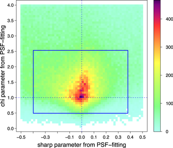
Figure 10. chi vs. sharp parameters from PSF-fitting (using DAOPhot) for transient candidates extracted from ≃30,000 difference images. Only candidates with  and S/N
  were used. The solid rectangle spans the 1–99 percentile range along each independent axis for candidates with a real-bogus machine-learned reliability score of
  (see Section 4.9.4 for details).
Download figure:
Standard image High-resolution imageTable 7. Transient Candidate Source Metrics and Features from PTFIDE
| Metrica | Description |
|---|---|
| xpos | X-image coordinate [one-based pixels] |
| ypos | Y-image coordinate [one-based pixels] |
| R.A. | J2000 R.A. [degrees] |
| decl. | J2000 Decl. [degrees] |
| magpsf | Magnitude from PSF fit [mag] |
| sigmagpsf | 1-σ uncertainty in PSF-fit magnitude [mag] |
| flxpsf | Flux from PSF fit [DN] |
| sigflxpsf | 1-σ uncertainty in PSF-fit flux [DN] |
| magap | Magnitude from aperture photometry [mag] |
| sigmagap | 1-σ uncertainty in magap [mag] |
| flxap | Flux from aperture photometry [DN] |
| sigflxap | 1-σ uncertainty in flxap [DN] |
| snrpsf | Ratio: flxpsf/sigflxpsf |
| sky | Local sky background level [DN] |
| nneg | Number of negative pixels in a 7 × 7 box |
| nbad | Number of bad pixels in a 7 × 7 box |
| distnr | Distance to nearest reference image extraction [arcsec] |
| magnr | Magnitude of nearest reference image extraction [mag] |
| sigmagnr | 1-σ uncertainty in magnr [mag] |
| arefnr | aimage (major axis rms) of nearest reference image extraction [pixels] |
| brefnr | bimage (minor axis rms) of nearest reference image extraction [pixels] |
| normfwhmrefnr | Ratio: (fwhm of nearest ref-image extraction)/(average fwhm of ref-image) |
| elongnr | Elongation of nearest reference image extraction (=arefnr/brefnr) |
| chi | Chi value from PSF fit |
| sharp | Sharpness value from PSF fit |
| nneg2 | Number of negative pixels in a 5 × 5 box |
| nbad2 | Number of bad pixels in a 5 × 5 box |
| magdiff | Magnitude difference: magap—magpsf [mag] |
| fwhm | FWHM from Gaussian profile fit [pixels] |
| aimage | Windowed rms along major axis of source profile [pixels] |
| aimagerat | Ratio: aimage/fwhm |
| bimage | Windowed rms along minor axis of source profile [pixels] |
| bimagerat | Ratio: bimage/fwhm |
| elong | Elongation = aimage/bimage |
| seeratio | Ratio: fwhm/(average fwhm of science image) |
| mindistoedge | Distance to nearest edge in frame [pixels] |
| magfromlim | Magnitude difference: diffmaglim—magpsf [mag] |
| ksum | Pixel sum of psf-matching kernel for image partition containing source |
| kdb | Differential background associated with psf-matching kernel estimate for image partition containing source [DN] |
| kpr | 5th–95th percentile range of pixel values in psf-matching kernel for image partition containing source |
| rbb | Real-bogus quality score from machine-learned vetting |
| stridc | Primary key from Stars table, if match is available |
| luidc | Primary key from LU (Local universe) table, if match is available |
| cvsidc | Primary key from CVs (Cataclysmic Variable Stars) table, if match is available |
| qsoidc | Primary key from QSOs (Quasi-Stellar Objects) table, if match is available |
| lcidc | Primary key from LCs (Light Curves) table, if match is available |
| rockidc | Primary key from Rocks (Asteroids) table, if match is available |
Notes.
aA majority of these are loaded into the candidates and features relational database tables (Section 5) to support trending and machine-learned vetting (Section 6). bThe real-bogus score is assigned following the loading of of all source metrics, features, and difference image-based metrics (Table 6). cThis is assigned following an association with a pre-loaded static database table (See Figure 13).4.9.5. Candidate Source Metadata and Features
In addition to the measurements and metrics from PSF-fitting (see above), the transient-candidate extraction tables are augmented with more metrics and features to support machine-learned vetting (Section 6). Most of these metrics are listed in Table 7. The shape metrics, for example aimage, bimage, elong, are computed by first executing SExtractor, then associating the extractions (with metadata) with those from DAOPhot above. Furthermore, the source metrics with names that end in nr in Table 7 refer to those of the nearest reference image source. These are assigned by associating the DAOPhot extractions with the input reference-image catalog, also originally from SExtractor.
Prior to implementation of the machine-learned vetting (Section 6), we resorted to simple one-dimensional cuts on a number of metrics in Table 7 in order to isolate those candidates as probably real transients. Unlike machine-learning, this involved no probabilistic classification of candidates into likely reals and bogus transients. It only provided a means to isolate candidates for further follow-up. The most powerful metrics and filtering logic we have found to label a candidate as "interesting" are as follows:
where the metric names on the left are defined in Table 7 and the corresponding thresholds (thressi) are specified by the –goodcuts input string with defaults defined in Table 2. The number of candidates that satisfy the above criteria per difference image are recorded as ncandgood in the QA output table (Table 6).
Figure 11 shows the number of transient candidates extracted from a collection of iPTF difference images acquired during late 2015 to early 2016, mostly at high galactic latitudes. These are shown as a function of the (point-source) FWHM and density of sources extracted from the science image using SExtractor to a fixed magnitude limit of  mag. Three different levels of candidate filtering are shown: first, the number initially extracted using the loose filtering described in Section 4.9.4 (ncandfilt); second, the number resulting from the simple one-dimensional cuts in Section 4.9.5 (Equation (49); ncandgood); and third, the number satisfying a machine-learned classification (realbogus) score of
  . This score corresponds to a false positive rate of
  % (see Section 6). A noteworthy feature in Figure 11(b) is the significant reduction in the number of initial candidates at relatively high source densities following simple 1D filtering (yielding ncandgood) or machine-learned vetting. In the end, the number that are visually scanned and subject to scrutiny before further follow-up are those that were machine-learned vetted (diamonds in Figure 11).

Figure 11. Number of transient candidates extracted per positive difference image as a function of (a) seeing FWHM and (b) integrated source density to  mag in the corresponding science image exposure. Extractions are from ≃30,000 difference images. To estimate the number of candidates per deg2, multiply the vertical axes by ≃1.56 deg−2. See Section 4.9.5 for details.
Download figure:
Standard image High-resolution imageWe have constructed animations of difference-images for two PTF CCD footprints made from image data acquired at  observation epochs. These can be accessed from the following URLs:
- 1.Field containing the M13 Globular Cluster: http://web.ipac.caltech.edu/staff/fmasci/home/idemovies/d4335ccd8f2movie.html
- 2.Field heavily used for supernova searches: http://web.ipac.caltech.edu/staff/fmasci/home/idemovies/d4450ccd2f2movie.html
Each epochal difference image is annotated with the two candidate numbers mentioned above (and shown in Figure 11): ncandfilt (or Nraw in the animation frames) and the number following machine-learned vetting above a realbogus (rb) cut:  .
.
4.9.6. Photometric Performance
One way to assess the photometric accuracy of the difference-image extractions is to examine the repeatability in their photometry under different observing conditions and/or input noise assumptions. Instead, we explore the photometric repeatability empirically at prior source positions across a stack of difference images generated from spatially overlapping exposures acquired over a range of observation epochs. Unfortunately we cannot perform this test on real flux-transients and variables because they intrinsically vary and will confuse repeatability statistics. We have resorted to exploring the scatter in photometric measurements from forced photometry on a list of prior source positions detected in a reference image co-add. The majority of the sources here will be non-variable and non-detected in the difference images. Even though undetected, their photometric residuals will persist, therefore providing sensitive probes of all random (and systematic) errors affecting the end-to-end difference image construction process in a relative sense across epochs. These residuals would arise from image misalignments, erroneous photometric-gain matching, flat-fielding errors, PSF-matching errors, Poisson noise from the science and reference images, and other instrumental/detector noise. At some level, there are also airmass-dependent color-refraction effects and astrometric scintillations.
It is important to note that these residuals will also include systematics from the forced-photometry process itself. For example, for forced PSF-fit photometry, these would include errors in the PSF estimates for each epochal image and their placement on the purported source positions in the difference image (the prior positions selected from the reference image). Therefore, the photometric variance inferred using forced PSF-fit photometry is likely to overestimate the true variance (or relative photometric accuracy) of detected transients in a difference image. As a reminder, the primary photometry measured for detected transients in PTFIDE is PSF-fit photometry (Section 4.9.2) where both flux and position are estimated per source. In forced photometry on prior positions, only fluxes are estimated.
Figure 12(a) shows an example of the robust rms in repeated forced PSF-fit photometry using 26,385 targets selected to R ≃ 22 mag from the reference image co-add. A portion of this reference image is shown in Figure 12(d) where it contains part of the North America Nebula. This was created from 20 good-seeing CCD images. Note that the complexity of this field is atypical of iPTF in general, but it provides a good test of image differencing in complex environments. Each reference-target position probes  difference images, generated from CCD images acquired over several months. The robust stack rms is based on half the 84.13–15.86 percentile difference in all photometric measurements per target position. This measure is relatively immune to outliers. This rms is shown as a function of reference image magnitude and can be interpreted in the context of real transients extracted from difference images as follows. A real transient with PSF-fit magnitude RPTF is expected to have a 1-σ uncertainty in the frequentist sense no larger than the rms shown in Figure 12(a) (i.e., relative to repeated measurement if the same event with the same intrinsic flux were re-observed).
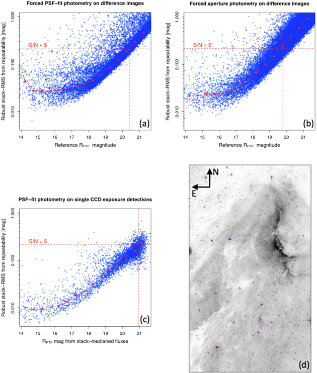
Figure 12. (a) rms in photometric repeatability from forced PSF-fit photometry on difference images overlapping a  CCD footprint falling on the North America Nebula. Prior positions used to seed the forced photometry are from the reference-image (co-add); (b) Same as (a) but using forced aperture photometry on the same positions; (c) rms in photometric repeatability from single-exposure PSF-fit extractions (not forced on prior positions) from a nearby CCD footprint; (d) A
  portion of the reference image containing part of the North America Nebula and from which source positions where used for (a) and (b). The vertical dashed lines in (a), (b), and (c) indicate the approximate 5-σ magnitude limits. The linked solid circles are binned medians.
Download figure:
Standard image High-resolution imageFigure 12(b) shows stack-rms estimates for the same prior target positions, but using forced aperture photometry instead. A fixed aperture of radius 6'' was used throughout. Comparing with the forced PSF-fit photometry in Figure 12(a), there are two noteworthy differences: first, aperture photometry results in a higher photometric precision at bright fluxes; and second, aperture photometry has a shallower limiting magnitude (5-σ limits are depicted by the vertical dashed lines). The converse of these applies to PSF-fit photometry. PSF-fit photometry lacks precision (relative to aperture photometry) at bright fluxes because knowledge of the underlying PSF is more critical. Systematic errors in the shape of the PSF-template and/or its centroiding will inflate errors in the photometry by a greater amount. Aperture photometry is more immune to these effects. The encouraging observation is that PSF-fit photometry leads to a fainter sensitivity limit (or more accurate photometry at fainter fluxes), in this case by ≃0.7 magnitudes.
For comparison, Figure 12(c) shows the performance of PSF-fit photometry extracted directly from a set of science image CCD exposures falling in a field flanking the North America Nebula. This has a background that is not as complex. As expected, the precision at bright fluxes is considerably higher that that inferred from forced PSF-fit photometry on difference images (Figure 12(a)). This is also higher than that achieved by forced aperture photometry (Figure 12(b)). Furthermore, the limiting magnitude from PSF-fitting on single CCD exposures is in general deeper (by at least 0.8 mag) than all other types of photometry performed for iPTF, for example SExtractor's mag_auto measure (Section 3.3; Ofek et al. 2012).
4.10. Forced, Sub-image (archival) Mode
PTFIDE can be executed in a mode where it operates exclusively on square sub-image cutouts. This is enabled if the –forced switch is specified. The science and reference image cutouts have a center (equatorial) position and side-length (pixels) specified by –forceparams (Table 2). In this mode, PTFIDE also expects as input a pre-computed (archived) PSF-matching kernel image FITS-cube, for example initially generated with suffix _pmtchkerncube.fits from a prior run of PTFIDE. The planes of this cube store the convolution kernels corresponding to partitions of the parent image (Section 4.7) and is supplied via the –kerlst input. This cube also stores metadata on each kernel, for example, the parent-image partition pixel ranges to which these apply, including all gain-correction factors. The appropriate kernel image for the parent-image partition containing the image cutouts (science and reference) is then applied (as in Section 4.8) to match their PSFs. Image-differencing is then performed on the cutouts.
Only a positive (science—reference) difference image stamp with accompanying uncertainty and mask image are generated in this mode. There is no source detection. Further outputs are generated if the debug switch was set (see end of Table 4). The purpose of this mode is to support later forced photometry on a target position of interest. This position would be the same used to generate the initial image cutouts. Operating on stamp cutouts using pre-existing kernel images is very fast, particularly when difference-images containing specific source positions over a historical observation range are needed. This avoids regenerating entire difference images, including all associated PSF-matching kernels and corrections. It also avoids archiving entire difference images in the first place.
5. Transients Database Schema
This section describes the schema and related workings of the iPTF Transients Database in current operations, along with how it will be improved for ZTF in future. Figure 13 depicts a simplified snapshot of the schema, in which each box represents a separate database table with a given name and some number of columns. The major table columns are listed. The columns in bold font are the table's primary keys. The columns in bold-italicized font are the alternate primary keys. The columns in regular font are not-null columns, and those in regular-italicized font are null columns (in which null values may also be stored). F.K. represents a foreign key and "1 1*.." indicates a relationship of one record to many records.

Figure 13. Schema design for the iPTF Transients Database in current operations. See Section 5 for details.
Download figure:
Standard image High-resolution imageThe Subtractions table stores a variety of metadata for both the positive and negative difference images generated for each processed CCD image. The boolean isdiffpos discriminates between the two subtraction types. Many of the QA metrics from PTFIDE defined in Table 6 are included in this database table. Associated with each record are the observation time (jd is the Julian date) and foreign-key database IDs of the corresponding field, filter, chip, reference image, and pre-processed science image. A stored difference-image filename contains the full pathname, and in its record, is accompanied by an MD5 checksum, a timestamp for when the record was created, and a status flag for whether the subtraction satisfied a number of QA criteria: status = 1 if so, status = 0 if not (see Section 4.8.2). Multiple versions of difference images are possible if the pipelines are rerun, and therefore the version number and vbest flag for which version is best (generally the latest) are also stored. The primary key for this table is subid, while the alternate primary keys are pid, isdiffpos, and version.
The Candidates and Features tables hold metadata for all transient candidates extracted from difference images with status = 1 only. The records in these tables store many of PTFIDE's source-based metrics and features, which are listed in Table 7. Included are null columns for storing the foreign-key database IDs of the closest positional matches to astronomical objects of interest (as discussed below). These are updated after the corresponding record is loaded, where a null value indicates either there is no match or no match was attempted. While candid is a unique candidate index assigned in sequence by the database, tblid is a relative number assigned to each candidate for a given difference image. The versioning mechanism in the Features table is not used at this time.
The RealBogus table stores the scores computed by the machine-learned classifier for all transient candidates (see Section 6). The RB score is a value in the range [0, 1] where a higher value indicates the candidate is more likely to be a real transient. Improved versions of the classifier are forthcoming, and a mechanism for tracking them in this database has been implemented.
The KnownRocks table contains the predicted positions (ephemerides) and magnitudes of all known numbered asteroids through the end of year 2019. The predictions are spaced 1 day apart. This table contains ≈400,000 asteroids and ≈1500 epochs for each, giving a total of ≈600 million rows. For each positive subtraction, the known rocks within its sky-footprint are found and loaded into the Rocks table. A 30'' cone search (accounting for uncertainty) is used to find the nearest rock to each candidate, and the corresponding rockid is updated in the Candidates record.
The Stars table holds the positions and magnitudes derived from PTF R-band reference-image catalogs for sources that have been classified to be stars by a star/galaxy classifier (Miller et al. 2016). Candidates are matched to stars in this table to within 1'', and the resulting Candidates record is updated with primary key strid of the match.
A typical database query would be for transient candidates within an observation-time and RB-score range, with an additional constraint that each be associated with at least another candidate (potentially from the same source) at approximately the same sky position, but with observation-times and magnitudes that differ by specified tolerances. Transients that have been spectroscopically confirmed and classified are inserted into the Transients table. The iPTF Transients Marshal, which is a web-based tool for analyzing lightcurves, is updated continuously with records from this table. Approximately 64 thousand classified transients are currently stored.
The database schema will be streamlined in future for ZTF so that it is scalable and more efficient. Sets of complete Candidates records will be fully constructed ahead of time for bulk database-loading. This will require the unique candidate IDs to be formed predictively rather than from a database sequence. Any redundant and unnecessary columns in the Features table will be eliminated. Also, the Candidates and Features tables may be combined into a single table. Partitioning the Candidates, Features, and perhaps other tables into child tables that isolate different observation-time ranges will also be considered, as this will allow for faster queries by taking advantage of constraint exclusion in the PostgreSQL database.
6. Machine-learned Vetting
The machine-learned vetting of sources is necessitated by the overwhelming number of artifacts produced by image subtraction and subsequently extracted during source finding. The true ratio of real astronomical sources (referred to as reals) versus artifacts generated by image subtraction (referred to as boguses) is unknown since the majority of sources extracted are unexamined. We estimate the bogus to real ratio for PTFIDE is typically greater than 10 to 1. This necessitates the use of automated systems to discriminate between boguses and reals in order to filter out unreliable candidates and prioritize detections for further study.
We refer to systems that perform this task as "RealBogus" systems, a term coined by Bloom et al. (2012). The use of machine learning for the vetting of astronomical transients extends back to PTF (Bloom et al. 2012). Machine learning systems are typically statistical classifiers that are able to score candidates on a spectrum from zero (bogus) to one (real). Classifiers are trained with annotated data exemplars as opposed to expert-specified rules. Three machine learning systems are currently in use for iPTF (Brink et al. 2013; Woźniak et al. 2013; Rebbapragada et al. 2015) for vetting outputs from the image differencing pipeline at NERSC. The results therefrom are combined to minimize missed detections. Machine-learned vetting is also being used for other surveys that use image differencing for transient discovery, for example, the Dark Energy Survey (Goldstein et al. 2015) and Pan-STARRS (Wright et al. 2015).
Here we briefly describe the construction and evaluation of the RealBogus system for PTFIDE and leave the details to a future paper.
6.1. Classifier Description
The RealBogus system for PTFIDE, like all its predecessors, is based on a random forest classifier. For an overview of random forests, see Breiman (2001), Hastie et al. (2009), and Masci et al. (2014). We use an ensemble of 300 trees trained on 10,000 real and 10,000 bogus candidates. The proportion of trees reporting a classification of real is reported as the candidate's score. Each candidate is described via a set of features that forms an input vector into the classifier. The current set of 89 features are outputs from PTFIDE and consist of both image-based and source-based features (Tables 6 and 7 respectively). This excludes irrelevant and trivial information such as source IDs, database counters, positions (i.e., R.A., decl.), and the constant photometric zeropoints.
Figure 14 shows a feature importance diagram that provides an estimate of the relative importance of each feature to the classification process. Only the twenty most important features are displayed. Despite the high number of features, the top two features for discriminating between real and bogus candidates are sigmagpsf (the 1-σ uncertainty in the PSF-fit magnitude) and status (a flag for whether the difference image satisfied a number of QA criteria; see Section 4.8.2). It is important to note that the relative feature importance ranking in Figure 14 does not account for any correlation between features. For example, the chi and sharp features are expected to be highly correlated. Removal of one of these features will still result in a good classifier, while removing both will not. I.e., the presence of either one but not necessarily both is important for overall classifier performance.
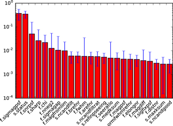
Figure 14. Relative importance of the first twenty most-important features. A higher "importance value" implies the feature is better at discriminating between real and bogus transients.
Download figure:
Standard image High-resolution image6.2. Training Data
The training data must be well sampled with respect to the true distributions of real and bogus candidates on any given night. The RealBogus system for PTFIDE benefited from predecessor systems at NERSC in that we could reprocess images containing real candidates discovered at NERSC and recover them with PTFIDE. We queried the NERSC database for all objects that were spectroscopically confirmed to be a supernova, variable star, gap transient, cataclysmic variable or nova. This resulted in 372 candidates. We augmented this set with data belonging to the lightcurves of these candidates at all observation epochs. This resulted in 15,168 real candidates in total. All images containing this candidate set were reprocessed with PTFIDE. Of these 15,168 candidates, 2153 were lost due to PTFIDE failures, of which 11 were spectroscopically confirmed. Of the remaining recoverable 13,015 candidates, we recovered matching transients for 11,075 (≃85.1%) with PTFIDE. 361 of these were spectroscopically confirmed of which we recovered 310 (≃85.8%). We reserved 10,000 of the 11,075 for training and reserved the remaining 1075 as an independent test set for final validation.
Bogus candidates are pipeline artifacts that must be sampled directly from the PTFIDE database. We randomly sampled 20,000 candidates exclusive of known reals and declare them as bogus. We reserve 10,000 for training and another 10,000 as an independent test set. Figure 15 shows an example of the various kinds of bogus transients extracted. Some are induced from bad or inaccurate upstream instrumental calibrations, while others are due to inadvertently unmasked detector glitches or artifacts from the optical system.
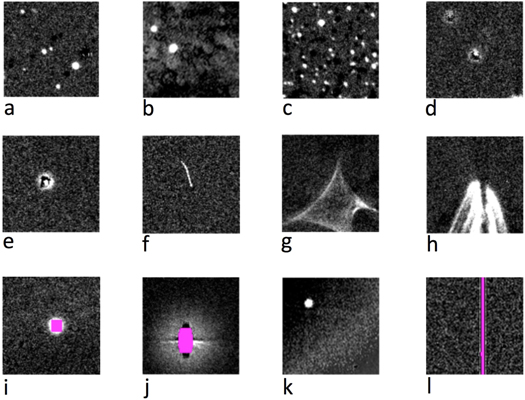
Figure 15. A sample of "bad" difference images with "bogus" transients. Their causes are as follows: (a) bad astrometric calibration; (b) bad photometricthroughput (gain) matching brought about by spatial variations in either atmospheric transparency or bad flat-fielding; (c) bad astrometric calibration in a high source-density field; (d) bad PSF-matching brought about by bad seeing and inability of the PSF-matching kernel to accommodate the disparity between science and reference image FWHM values; (e) same as (d); (f) moving-object streak; (g) bright-source halo artifact; (h) bright-source glint; (i) incomplete masking of a saturated source; (j) incomplete masking of a bright source and its halo and charge bleed artifacts; (k) bad background matching and photometric-throughput (gain) matching; (l) incomplete masking of the edges of a bad-pixel column.
Download figure:
Standard image High-resolution imageIt is impossible to ensure the purity of our samples without examining each candidate individually. The bogus set may include missed detections while our labeled sets of real candidates may contain artifacts. Future work includes plans to assess training set contamination via a machine learning technique called active learning (e.g., Richards et al. 2012).
6.3. Evaluation and Setting Decision Thresholds
We have two methods of evaluation. The first is to use ten-fold cross-validation in order to form a receiver operating characteristic (ROC) curve that measures the false positive rate (FPR) and false negative rate (FNR) at a continuum of decision thresholds from 0 to 1. In ten-fold cross-validation, all 20,000 labeled examples (exclusive of the independent test sets) are randomly split into 10 groups, where one fold is held out as the test fold and the classifier is trained on the remaining nine. The test fold is rotated and the predicted outcomes from the ten classifiers are averaged across the folds. Methodologically, cross-validation usually assumes examples are independent and identically distributed. That is not the case here, since light curve observations from the same source (especially variable stars) may span both the training and test folds. We use cross-validation as a guide when comparing competing versions of the classifier, rather than for assessing the system's overall performance. In fact, cross-validation is prone to overfitting if the labeled population does not well represent the general population of candidates. Figure 16 shows the ROC curve for the classifier using cross-validation, where the y-axis shows the true positive rate (TPR = 1 −FNR). The FNR at 1% FPR, the maximum FPR tolerated by the science teams, was 3.51% from cross-validation.
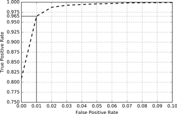
Figure 16. Receiver operating characteristic (or ROC) curve. See Section 6.3 for details.
Download figure:
Standard image High-resolution imageThe second evaluation of the system looks at score distributions on the two independent test sets of real and bogus examples. This gauges performance and determines the system's decision threshold. Candidates that score above the decision threshold are presented to the science teams for inspection, while those below will likely remain unexamined. We classify the candidates in the test set of randomly selected candidates and note the threshold that admits only 1% of the set as false positives. Similarly, using the independent test set of known reals, we classify this set and note the threshold that admits only 5% as false negatives (or missed detections). The thresholds resulting in a 1% FPR and 5% FNR were 0.735 and 0.724 respectively. As a result, the decision threshold for the RealBogus classifier was set to 0.73. Figure 17 shows the distribution of RealBogus scores obtained from PTFIDE run on iPTF data. As seen in Figure 17(a), the decision threshold of 0.73 corresponds to a plateau followed by a knee in the distribution above which the FPR falls below 1%.
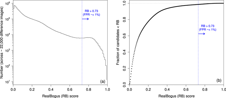
Figure 17. (a) Histogram of the RealBogus (RB) scores for transient candidates extracted from ≃22,000 R-band (positive) difference images down to S/N ≃ 4. These are from exposures acquired from 2015 December to 2016 February, mostly at moderate to high galactic latitude; (b) Cumulative fraction as a function of RB. See Section 6.3 for details.
Download figure:
Standard image High-resolution image
6.4. Further Work on Machine-learned Vetting
Areas of future work include plans for identifying and eliminating training set contamination. We have built an active learning prototype that identifies candidates that are likely mislabeled, and present those to the science teams for cleaning. We have also developed a new way to randomly sample against the PTFIDE candidates database to ensure our bogus sample is not overly biased toward certain types of artifacts and is representative of the full distribution of observing conditions. Finally, we have used machine learning to analyze the frequency of certain types of bogus artifacts produced by PTFIDE in order to understand the software and faciliate improvements. Details on these methods will be published in a forthcoming paper.
7. Lessons Learned
The iPTF realtime processing system has evolved considerably over the last few years through feedback received from the various science programs. The system was developed by a small team with limited resources. Communication between the development team and users of the products was paramount. The success of a large astronomical survey requires (i) a clear definition of the science goals and deliverables needed to achieve these; (ii) a tractable system engineering plan to enable (i), given the available resources. Below we list some of the challenges and pitfalls encountered over the course of development and how these were addressed. We also present thoughts on how specific aspects could have been improved if resources allowed.
- 1.Tuning and optimization of all processing components is an iterative process that requires real on-sky data acquired with your survey instrument. Do not rely on the commissioning period to optimize everything to perfection. Resources (and schedule) are limited. More eyes on the data, the better, and this can only occur by harnessing the expertise of the scientific community. Immediate visibility to data products is therefore crucial in the early phases of the survey.
- 2.Implement offline versions of your primary production pipelines to allow for experimentation and ongoing tuning. This ensures minimal disruption to the production system that is serving users. Communicate all planned updates in advance and only deploy when the stakeholders have confirmed and understood the updates.
- 3.Allow versioning control of all pipeline software parameters and instrumental calibrations together with the software versions they were optimized for. This will allow for easier traceability and reproducibility of specific science products in future.
- 4.Have a well defined quality-assurance plan for the entire observing and data-processing system. This entails implementing QA metrics for each subsystem and a means to communicate these across all subsystems. For example, implementing automated checks at the raw-data level (close to realtime) alerts the team of bad data and that no products are expected downstream. A modular and visible end-to-end QA/alerting system allows for easier accountability of missing products, traceability of errors, and recovery.
- 5.Related to the previous point, routine monitoring should include overall performance of the network, data-transfer rates, and all aspects of the compute cluster.
- 6.Assign ownership and responsibility of key components of the system to individuals of the team. For example, this may consist of collecting performance metrics, analysis reports, and/or providing feedback for improving aspects of the data-processing system. Having all communication channels defined at the outset will allow priorities to be better managed.
- 7.Time-domain surveys are dynamic, literally. For example, science goals or their priorities may change over time in response to scientific outcomes or analyses early in the survey. Goals may also change in response to unforeseen problems in instrumentation, hardware, and/or algorithmic or processing details. Be prepared to adapt. Modularity in all pipeline software and hardware components to accomodate change and growth is therefore crucial.
- 8.In the context of realtime discovery using image-differencing, the accuracy of upstream calibrations is crucial. This primarily refers to astrometric and photometric calibration. Flat-fielding in particular is important for the latter. Proper trending and QA of all calibration products prior to use is therefore necessary to avoid a flood of false-positives downstream. Early notification of bad calibrations and a means to either recreate them on-the-fly or fallback to archived versions should be planned.
- 9.Have a plan to assess the overall performance of image-differencing and transient-discovery over the course of the survey. This may involve for example tracking the relative efficiency and reliability of candidates extracted from pre-defined survey fields known to contain a good statistical sample of variable stars. Alternatively, one could inject synthetic episodic transients for offline analysis. The important thing is that the appropriate metrics and methodologies to enable this monitoring be identified and implemented prior to commencement of the survey.
- 10.Image-differencing is a game of (i) minimizing false-positives at the expense of also maintaining a low false-negative rate, and (ii) maximizing the photometric accuracy. These sensitively depend on the initial extraction S/N. The power of using machine learning to probabilistically classify candidates into either real or bogus cannot be overstated. False-positives are inevitable. We advise setting a maximum tolerable threshold for their occurence to enable tuning of the relevant extraction and scoring thresholds. These will evolve as algorithms and software improve.
- 11.The efficacy of a machine-learned vetting infrastructure crucially depends on the data it was trained on (in the context of supervised learning). This should be kept in check over the course of a survey according to the different science applications and possible changes in survey design. For example, if a decision is made to survey more of the galactic plane, the machined-learned classifier should be retrained accordingly using data from the same region. This minimize biases when predicting the reliability of transient candidates.
- 12.A supervised machine-learned classifier will have been trained on products from a specific version of pipeline software. Any algorithmic or parameter changes in the pipeline usually requires a retraining of the classifier. This dependency will incur a delay in the software delivery cycle and must be accommodated. We have not yet streamlined this delivery and integration process since classifier (re)training can be time-consuming. We advise that any classifier-retraining be performed on a stable version of the pipeline software. Both can then be updated as shortcomings are identified during the survey.
- 13.Plan on reprocessing any or all of your data, for example, to recover from failures in processing and/or hardware outages. This also enables one to regenerate products for a future archive using a consistent set of pipeline parameters and software. These may have evolved over the course of the survey.
8. Enhancements and Future Work
A number of shortcomings were identified over the course of development of the iPTF Discovery Engine. Some of these are at the algorithmic level and some relate to data management practices. In 2017, iPTF will be replaced by the Zwicky Transient Facility (ZTF; see Section 1). The higher data rates and volumes will require a redesign of some of the subsystems to minimize processing latencies and the delivery of transient candidates for scanning. The planned upgrades are as follows:
- 1.Improve the efficiency of loading and retrieval of candidates into/from the Transients Database described in Section 5. The plan is to periodically construct lists of pre-machine-vetted candidates ahead of time at intervals throughout a night and batch-load them. Source features and metrics will be consolidated into single (flatter) database tables. We will also consider retaining only candidates and associated metadata for the last 30 nights or more to enable more efficient near real-time discovery and lightcurve generation. Older transient candidates will roll-off to a growing archival database. The reason for this is to keep the number of candidate records for active-querying (close to their discovery epoch) relatively small.
- 2.Transient candidates and image-cutouts for human scanning will need to be delivered for external viewing using pre-defined (or cached) database queries submitted by an automated process at regular intervals throughout a night. Currently for iPTF, there is no limit on how many queries can be submitted. Having many scanners submit similar queries in an uncoordinated manner has led to severe bottlenecks.
- 3.Astrometric calibration needs to be made more robust against changes in source density, seeing, depth, atmospheric refraction, and telescope tracking. This includes the ability to properly model and capture time-dependent distortion effects from the optical system and atmosphere.
- 4.Absolute photometric calibration will need to be performed on a per-image basis in the realtime pipeline. The use of PSF-fit photometry in particular is paramount. PSF-fitting will automatically account for seeing variations and regions with high source-confusion through its de-blending ability. This will ensure that photometric zeropoints can be accurately determined for a larger fraction of the images. As discussed in Section 4.2.1, the zeropoints are refined using big-aperture photometry to enable more accurate gain-matching prior to image-differencing. This method is fragile and has not been reliable.
- 5.Extend PTFIDE to include some of the optimal methodologies for co-addition, image-differencing, source detection, and photometry presented in the detailed study by Zackay et al. (2016).
- 6.Consider using pre-classified star catalogs constructed initially from reference image catalogs (e.g., via machine-learning) to properly seed inputs for deriving PSF-matching kernels.
- 7.Consider dynamic updates to reference image products as the survey proceeds in order to use the best-quality epochal data acquired to date. In other words, the reference-image library can be progressively refined to ensure optimal image-differencing.
9. Conclusions
We have described a transient-discovery engine (IDE), currently in use to support near real-time discovery for iPTF at IPAC/Caltech. A refined version will be used for ZTF in future. Guided by previous implementations of the image-subtraction problem, this paper reviews our algorithms, optimization strategies and machine-learned vetting scheme. Once tuned, the pipeline requires little intervention and is resilient to bad input data and/or inaccurate instrumental calibrations. Our development approach was to make all processing steps as modular as possible to allow for easier debugging and tractability.
Our goal has been reliable transient discovery and robustness. The methods were refined using the knowledge gained from 6+ years of archived science-quality PTF data. The elements we find that are most crucial to image-differencing performance, and hence the efficiency and reliability of transient discoveries are: (i) astrometric calibration; (ii) flat-fielding; and (iii) related to this, photometric calibration (either relative or absolute). Having these calibrations optimized (in the maximal S/N sense) paves the way to more accurate PSF-matching and image-differencing. This also relieves the amount of work needed downstream to weed out false positives, by both human and machine. Despite differences in the details of instrumentation, image quality and/or survey design, IDE provides a testbed for future large time-domain surveys.
This work was funded in part by the iPTF and ZTF projects at the California Institute of Technology. iPTF is a partnership led by the California Institute of Technology and includes the Infrared Processing & Astronomical Center; Los Alamos National Laboratory; University of Wisconsin at Milwaukee; Oskar-Klein Center of the University of Stockholm, Sweden; Weizmann Institute of Sciences, Israel; University System of Taiwan, Taiwan; the Institute for Physics & Mathematics of the universe, Japan; Lawrence Berkeley National Laboratory and the University of California, Berkeley. ZTF is funded by the National Science Foundation under grant no. AST-144034. M.M.K. acknowledges support from the National Science Foundation PIRE GROWTH award. A.A.M. acknowledges support for this work by NASA from a Hubble Fellowship grant: HST-HF-51325.01, awarded by STScI, operated by AURA, Inc., for NASA, under contract NAS 5-26555. Part of the research was carried out at the Jet Propulsion Laboratory, California Institute of Technology, under a contract with NASA.
The pipelines use a number of software packages from other institutions and past projects (see Table 1), for which we are indebted. Portions of the analysis presented here made use of the Perl Data Language (PDL) developed by K. Glazebrook, J. Brinchmann, J. Cerney, C. DeForest, D. Hunt, T. Jenness, T. Lukka, R. Schwebel, and C. Soeller and can be obtained from http://pdl.perl.org.
PDL provides a high-level numerical functionality for the Perl scripting language (Glazebrook & Economou 1997).
We thank the anonymous referee for valuable comments that helped improve the quality of this manuscript.
Facility: PO:1.2m. -
Footnotes
- 8
For a list of all publications to date, see http://www.ptf.caltech.edu/iptf.
- 9
Source code, instructions for installing external dependencies and examples with test data are available at http://web.ipac.caltech.edu/staff/fmasci/home/ptfide.
- 10
FITS stands for Flexible Image Transport System; see http://fits.gsfc.nasa.gov.
- 11
Source code, instructions for installing external dependencies and examples with test data are available at http://web.ipac.caltech.edu/staff/fmasci/home/ptfide.
- 12
- 13
These will be affected by source confusion in crowded fields. In future, we will use PSF-fit photometry from both images, that includes source-deblending.
- 14
- 15
This ratio is used if the reference image was convolved, otherwise the inverse of this ratio is used.
- 16
This ratio is used if the reference image was convolved, otherwise the ratio is refconvseeing/refinpseeing.
- 17