


Abstract
We consider the effect of introducing a small number of non-aligning agents in a well-formed flock. To this end, we modify a minimal model of active Brownian particles with purely repulsive (excluded volume) forces to introduce an alignment interaction that will be experienced by all the particles except for a small minority of 'dissenters'. We find that even a very small fraction of dissenters disrupts the flocking state. Strikingly, these motile dissenters are much more effective than an equal number of static obstacles in breaking up the flock. For the studied system sizes we obtain clear evidence of scale invariance at the flocking-disorder transition point and the system can be effectively described with a finite-size scaling formalism. We develop a continuum model for the system which reveals that dissenters act like annealed noise on aligners, with a noise strength that grows with the persistence of the dissenters' dynamics.
Export citation and abstract BibTeX RIS

Original content from this work may be used under the terms of the Creative Commons Attribution 3.0 licence. Any further distribution of this work must maintain attribution to the author(s) and the title of the work, journal citation and DOI.
1. Introduction
Flocking models inspired by the seminal work of Vicsek [1] have been shown to describe organization and collective motion on many scales, from self-motile colloids [2] to bacteria [3], bird flocks [4] and human crowds [5, 6]. In these models individual active agents are described as self-propelled particles that tend to align their direction of motion with their neighbors, in the presence of noise in the angular dynamics that effectively describes 'mistakes' in the alignment. These models exhibit a non-equilibrium phase transition from a disordered state to a flock where on average all agents are moving in the same direction, with long-range order in the particle velocities. The transition occurs upon decreasing the strength of the noise or increasing the density. The order of the transition in the original Vicsek model of point-like particles has been the subject of a long-standing debate, but it has now been established that the transition is first order, with coexistence and hysteresis [7–9].
Recent work has begun to consider the effect of disorder either present in the environment in the form of physical obstacles to the motion [10–14] or arising from variations in the properties of individual agents or their ability to align with neighbors [15–19]. Both environmental disorder and disruptions in alignment rules were found to destabilize the flocking state, in agreement with observations in bacteria and insect swarms, where a fraction of individuals with a decreased production of signaling compounds or pheromones that promote collective behavior can disrupt organization.
In this paper we consider the effect of a fraction of non-aligning agents or 'dissenters' on a well-formed flock. Previous authors have examined the effect of non-aligning agents on a flock that is made cohesive by attractive interactions [19]. In this case, provided the cohesiveness is not too strong, aligning agents are able to expel non-aligners and reorganize in smaller, but still cohesive flocks. Our work, in contrast, focuses on the case where the self-propelled agents only experience repulsive interactions due to volume exclusion, in addition to alignment, but no attractive forces. We find that in this case even a very small concentration of dissenters disrupts the flocking state. Additionally, this behavior depends only weakly on the combined packing fraction of aligners and dissenters, provided the packing fraction is large enough that the pure system with no dissenters is deep into the flocking state. A striking behavior is found when comparing the effect of dissenters to that of an equal concentration of static obstacles (figure 4). A small concentration of static obstacles only disrupts the orientational order locally, creating small wakes of misaligned particles downstream of the obstacles, in qualitative agreement with experiments in colloidal rollers [12]. In contrast, the same concentration of motile dissenters completely disrupts the flock. Using a hydrodynamic model of a mixture of aligners and dissenters, we show that motile dissenters, in contrast, provide an effective annealed disorder with finite-time correlations that can rapidly disorder the flock. This observation could have implications for crowd control, as it suggests that randomly distributed, but motile dissenters with persistent dynamics could be very effective at dispersing crowds in high risk situations (see [5, 6] for studies of human 'flocks').
In the following we begin in section 2 by describing our system—a mixture of self-propelled aligners and dissenters based on a minimal model of active Brownian colloids. We then briefly summarize the physics of the pure case (aligners only) and identify values of the parameters that result in a strongly ordered flock. This system is then disrupted by adding a small number of dissenters, which succeed in breaking up the alignment. The effect of these dissenters is quantified in section 3 by considering high-precision simulations for several packing fractions, which leads us to identify the fraction p of dissenters required to disrupt the flock as  , independent of the total density of active particles, provided again the latter is large enough to set up the flocking state. The role of the range of the alignment interaction is discussed in appendix A. In section 4 we compare the dramatic effect of motile dissenters to the much weaker disruption caused by static obstacles. In section 5 we compute the correlation length of the system and use it as the basis of a finite-size scaling (FSS) study to try to determine the order of the transition and its critical parameters. Finally, in section 6 we examine the continuum equations for a mixture of aligners and dissenters (derived in appendix C). We show that dissenters act like annealed, but time-correlated, disorder and provide an analytical estimate of the shift they induce on the flocking transition.
2. Model and simulations
We consider a minimal model of repulsive active Brownian particles (ABPs) [20–22] with an additional feedback mechanism that tends to align the direction of self-propulsion to the local velocity field [23, 24]. The system is composed of N particles of radius a in a two-dimensional box of size L2 with periodic boundary conditions. A particle i is characterized by its position  and an angle
  that defines the direction of self-propulsion.
The dynamics is then defined by coupled Langevin equations


The first term in the translational equation of motion represents the self-propulsion along a direction  . The second term is an excluded volume interaction, which we model with a soft repulsive force,
  if
if  and
and  otherwise. The rotational equation of motion includes a noise term, with a random torque
  with zero mean and correlations
  . In addition to these fluctuations, the polar angle
  evolves due to a torque proportional to the angle between
  and the instantaneous direction of motion
  , defined by
  . In other words, as the particles collide their orientations relax towards the direction of the local velocity field with a lag time τ and a Gaussian noise of variance
  .
.
The model described by equations (1) and (2) experiences a flocking transition if the noise is low enough (i.e., if  is large compared to τ) or if the density is increased at fixed noise [23, 24].
Notice that alignment can be modeled in several ways—see, e.g. [25] for an alternative approach with active polar hard disks—but the results presented herein are not very sensitive to the details (see appendix A for an example with a Vicsek-type alignment [1]). Likewise, whether the repulsive interaction is introduced with a spring force or with a harder potential (such as WCA) should not have a noticeable effect.
In our simulations we take the radius a = 1 of the disks as our unit of length and set  , taking the interaction time
  as our temporal unit. The alignment lag is also set to
  . The self-propulsion speed is v0 = 0.01, which is small compared to
  to prevent particle overlap. The noise is set to
  : this results in a persistence length of
  and generates a strong alignment. We will change the packing fraction ϕ in order to transition from the low-density disordered state to the high-density flocking state.We consider system sizes of up to L = 400, which, for a typical packing fraction of
  , results in about 20 000 disks.
Now we introduce a second species in the system. Out of our N disks,  will still be aligners, described by equations (1) and (2). The other pN disks will be dissenters: they have the same characteristics as the aligners, except for the alignment interaction. In other words, their equations of motion are just those of standard ABPs:


In the following we consider simulations of our combined system of aligners and dissenters for different values of p and ϕ.
3. Effect of the dissenters
Even a very small fraction p of dissenters can have a dramatic effect on the system. This is demonstrated in figure 1, where we follow the time evolution of the system before and after introducing dissenters. In particular, we consider the average velocity of the system as the flocking order parameter,

Clearly V = 1 if all the disks are moving in exactly the same direction and V = 0 if their orientations are random.

Figure 1. Effect of introducing dissenters in a flocking system. The figure shows the time evolution of the order parameter V, equation (5). The system is prepared without any dissenters and is let to form a flock. At time  , we remove the alignment interaction from 3% of the particles (i.e., turn them into dissenters). The flock is dispersed very quickly. Two snapshots show the state of the system just before and just after introducing the dissenters. Each particle is plotted with a color representing the cosine of its angle of motion.
Download figure:
Standard image High-resolution imageWe first consider the pure system with p = 0, where all the particles experience the alignment interaction. In the initial configuration the positions and orientations of the particles are random but, as time goes on, a stable flock develops, as evident from the growth and saturation of V around V = 0.91 shown in figure 1. At time  , we turn 3% of the particles into dissenters, i.e., we switch off their alignment interaction. The effect on the system is very strong and fast: the flock is destroyed in a very short time (shorter than what it took to form originally).
Figure 2 gives a more general picture by considering the steady-state value of V for many values of p and ϕ. For each pair  we follow the system up to a time
  . We denote by
  the ensemble average in the steady state of an observable O, which we estimate numerically by averaging over the last half of our simulation (the time needed to reach the steady state is orders of magnitude shorter). The errors are estimated with a jackknife procedure (see, e.g., [26]) from the fluctuations over 100 independent runs for each set of parameters. This method allows us to compute errors in nonlinear functions of averaged quantities such as the susceptibility. Unless we say otherwise, all of the results in this paper are for a system size L = 200.
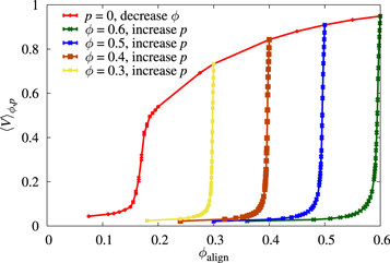
Figure 2.
 against the packing fraction of aligners ignoring the dissenters,
  . The red curve shows the flocking transition in the pure case (no dissenters, p = 0), as the system is diluted by changing ϕ. In the other curves we consider a fixed total packing fraction ϕ and slowly increase the fraction p of dissenters until the alignment is destroyed.
Download figure:
Standard image High-resolution imageIn order to plot all the data in the same graph and also to prove that the effect of the dissenters is much stronger than that of simply diluting the system, we define as  , the packing fraction of aligners ignoring the dissenters. The red curve in figure 2 refers to the pure system, where we keep p = 0 and decrease the total packing fraction (
 . As we can see, with our parameters we need a rather strong dilution in order to break our flock and cross over to the disordered state. In contrast, in each of the other curves we fix the total packing fraction ϕ and change
  by slowly increasing the fraction p of dissenters. In agreement with figure 1, we see that a very small value of p is enough to destroy the flock. The behavior does not seem to depend much on the value of ϕ.
To make this statement more quantitative we plot in figure 3 the order parameter normalized to its value at p = 0,  , as a function of p. All the curves collapse on top of one another, showing that (i) a very small fraction of dissenters is enough to completely disrupt the alignment and that (ii) this fraction does not depend on the density of the system. To locate the transition point, we consider the fluctuations of the order parameter,

We shall refer to χ as the susceptibility of the system, in analogy with equilibrium systems where equation (6) is an expression of the fluctuation–dissipation theorem [26]. As we can see in the inset of figure 3, χ has a maximum for  , which signals the finite-size crossover between the ordered and disordered phases. We will make this statement more precise below, where we outline a FSS study.
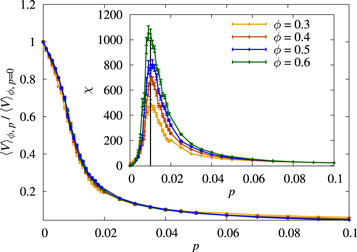
Figure 3. For the data with variable p in figure 2, we plot  , normalized by the value for p = 0 for each packing fraction. The curves for different ϕ collapse, showing that the effect of the dissenters does not depend on the density of the system. Inset: we plot the susceptibility (6) for the data in the main panel, whose peak at
  marks the crossover between the flocking and disordered phases.
Download figure:
Standard image High-resolution imageIt is interesting to compare this critical fraction of dissenters of  to the corresponding value for the finite cohesive flocks studied in [19]. In the latter, considering the limit of large inter-agent cohesiveness, typical values of the critical fraction of dissenters are around
  (see figure 1 in [19]). This fraction can even be further increased by lowering the cohesiveness, which allows aligners to expel dissenters and reorganize into several flocking clusters.
4. Static obstacles
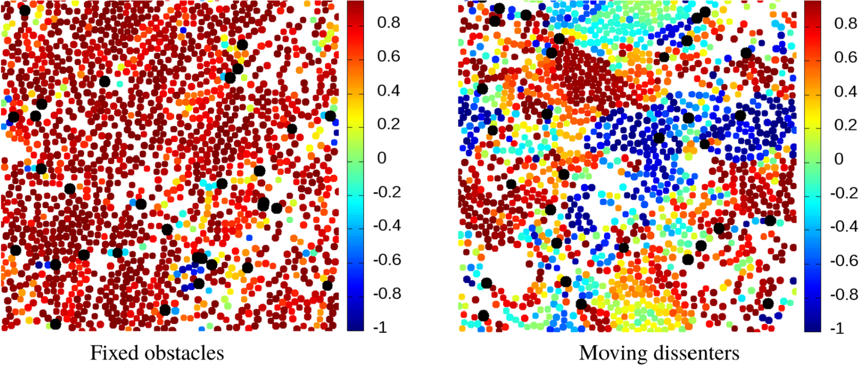
The effect of passive obstacles in a flocking system has been considered before using different models [10, 14]. In this section we show that our active dissenters are much more efficient at disrupting the alignment than static obstacles. This contrast is illustrated in figure 4, which shows snapshots of our model system with dissenters ( , p = 0.03) in the left panel and a system where the dissenters have been replaced by the same concentration of static obstacles (right panel). These obstacles are just immobile disks of the same radius as our active particles. The collisions of the aligners with the static obstacles are controlled by the same repulsive force that controls their interaction with motile dissenters. As we can see, for this fraction of static obstacles the system still maintains a high degree of alignment, while the system with dissenters is completely disordered.
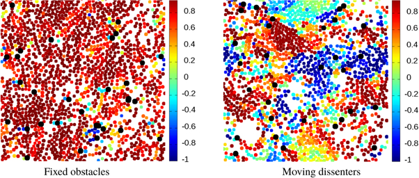
Figure 4. Snapshots of two systems with  in the steady state. In the left panel we have a fraction p = 0.03 of static obstacles, while in the right panel we consider the same number of moving dissenters. Both images are for L = 100. Aligners are color coded according to the value of
  , as indicated in the color bar. Obstacles or dissenters are shown in black and with size slightly larger than their actual size.
Download figure:
Standard image High-resolution imageThe difference between passive obstacles and dissenters is quantified in figure 5, which compares the order parameter and susceptibility for systems with static obstacles (blue) and moving dissenters (red). For the model with static obstacles, the peak is at  , in contrast with
  for the dissenters. In other words, one needs approximately five times as many static obstacles as dissenters to have an equally disruptive effect.
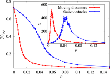
Figure 5. As in figure 3, but now we compare, for  , the effect of introducing dissenters (red curve) with that of introducing static obstacles (blue curve). The obstacles are much less efficient at breaking up the flock, as evinced by the very noticeable shift in the peak of the susceptibility and in the slower decay of
  .
.
Download figure:
Standard image High-resolution imageThe contrast between static obstacles and motile dissenters is probably due to the latter effectively providing an annealed disorder with finite-time correlations, in contrast to the weak quenched disorder of static obstacles. The persistent movement of the dissenters effectively gives them a greater cross section. We have tried to support this intuition with a continuum model presented in the following, see section 6.
5. The correlation length and FSS
Thus far we have presented essentially an exploratory study of a minimal model of flocking particles with dissenters. We have seen that a very small number of these non-aligning particles (about 1%) is enough to disrupt the flock. But this effect was observed for a single system size (L = 200). In order for this result to be considered a proper (non-equilibrium) phase transition, we would need to show that the effect of the dissenters is stable as we change the system size.
To this end, we have carried out additional simulations with L = 100, 400 for the system with dissenters and  . As we mentioned before, the peak in the susceptibility signals the finite-size crossover between the disordered and the flocking phases. When the system size is increased, this crossover region becomes narrower and narrower, as the crossover turns into a phase transition in the thermodynamic limit. To leading order, the position of the peak should evolve as

where A is a constant, ν is the correlation-length critical exponent and pc is the transition point. This behavior is qualitatively reproduced in our figure 6—top. In principle, we could fit the data in this plot to extract the critical parameters ν and pc. Unfortunately, with only three system sizes such a simultaneous fit for two parameters is not viable.
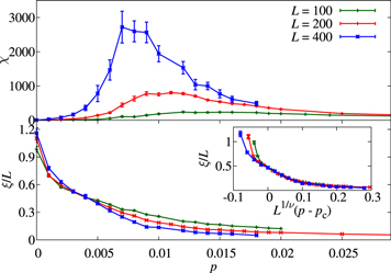
Figure 6. Scaling in the system with dissenters for  . Top: we plot the susceptibility χ, equation (6), for
  . As we increase L, the position of the peak shifts slightly to a lower p and its height grows. Bottom: correlation length of the particle orientation in units of the system size. The curves for different values of L intersect at
  , marking a second-order phase transition. Inset: scaling plot of the correlation length using
  and
and  .
.
Download figure:
Standard image High-resolution imageA better way to analyze a phase transition is to use the system's correlation length ξ. We begin by considering the spatial autocorrelation of the particle orientation:

In order to evaluate this quantity, we first discretize the system in a lattice with cells of size 2 × 2. The orientation  of cell
  is just the average of all the
  of particles in that cell. Then we evaluate

which is just the Fourier transform of  . From F we can compute the second-moment correlation length [26, 27],

where  is the smallest non-zero wavevector.
In a second-order phase transition the system is scale invariant, so the correlation length behaves as

In other words, if we plot  for our different system sizes, the curves will intersect at the transition point. We have done this in the bottom panel of figure 6, which shows that the system is indeed scale invariant, with a critical point of
  . In addition, we can find ν by looking for the value that produces the best collapse in (11). With our data, this is obtained for
  (although we cannot obtain a very precise determination). This scaling plot is shown in the inset to figure 6. Notice that the points for p = 0 are already out of the FSS region and do not collapse but this is expected, because these points are deep into the ordered phase, where F(0) diverges. These values of ν and pc are consistent with our data for
  and equation (7).
Our simulations show evidence of a continuous flocking transition. On the other hand, it has been established recently that the flocking transition in the pure Vicsek model is first order, with coexistence and hysteresis [7–9]. At the level of a continuum description the first order nature of the Vicsek flocking transition arises from the density dependence of the term linear in polarization in the polarization equation. In contrast, in models where the alignment is with topological neighbors rather than nearest neighbors, this term does not depend on density and the transition is continuous [28, 29]. In our model the alignment with the particle's own velocity is density dependent and we would therefore expect the transition to be first order. On the other hand, establishing the first-order nature of the flocking transition of point particles in the Vicsek model has required simulations with very large numbers of particles [8], with a crossover size that depends on the details of the model and parameters [7]. Below that crossover there is a wide range of system sizes where the transition looks continuous and FSS holds [30, 31]. When steric repulsion is included in the model, it becomes even harder to see clustering and band formation—the hallmark of the first order flocking transition (see appendix B)—as the fact that particles cannot overlap forces them to distribute more uniformly throughout the system. In fact, to the best of our knowledge, all studies of the flocking transition that find a first-order behavior have been carried out with point particles. Indeed, we have found that in the presence of both dissenters and static obstacles density fluctuations are much weaker in our model that includes steric repulsion that in a model of point particles of the type studied in [17]. We show examples of this different behavior in appendix B.
It is therefore likely that the scaling behavior observed in our work is a finite-size effect, and that for large system sizes the transition is first order. Unfortunately, with numerical simulations alone it is impossible to differentiate between an asymptotic regime and a pre-asymptotic one that would have a crossover at very large system sizes, well beyond those relevant to practical applications such as human crowds.
6. Continuum model
To gain insight on the picture emerging from our simulations, we have developed a continuum model that describes the system on length scales large compared to the particle size and time scales long compared to those controlling the microscopic dynamics. In this limit we describe the mixture of flocking (aligning) and dissenter agents in terms of the local number density of aligners and dissenters at position  and time t,
  and
and  , respectively, and the corresponding polarization densities
  and
and  . In this continuum model the net polarization
  serves as the order parameter for the flocking transition.
6.1. Hydrodynamics of a mixture of aligners and dissenters
The continuum equations have been derived via a standard coarse-graining procedure for a simplified continuous-time Vicsek model where all agents are treated as point particles that align their polarization to that of of their neighbors (see, e.g., [32]). The derivation is outlined in appendix C. We stress that the model used for the derivation of the hydrodynamic theory differs from the one used in the simulations as it considers point particles that align with the mean polarization of their neighbors, not with their own velocity. While the form of the hydrodynamic equations does not depend on the specific form of the microscopic dynamics, the latter does of course affect the expression of the parameters in the equations. The use of a continuous-time Vicsek model greatly simplifies the algebra. In addition, the assumption of point particles allows a direct comparison of the effect of dissenters with that of static obstacles as of course point static obstacles would have no effect on the organization of the aligners. The continuum equations obtained in appendix C are given by
where for generality we have distinguished the self-propulsion speed vD of dissenters from that of aligners given by v0. Here we have added a white noise term  with zero mean and correlations
  , needed to compute correlation functions, and we estimate
  . The polarization decay rate
  changes sign at a critical density
  and
and  . For the microscopic model described in appendix C.1, the various parameters in equation (12) are expressed in terms of the rotational diffusion rate Dr and the rate J at which particles align with their neighbors' polarization (see equation (C.1)). Although the alignment interaction used in the derivation of hydrodynamics differs form that employed in the numerical simulations described in equations (2), both models exhibit a flocking transition driven by alignment at low noise and high density, and we can estimate
  . This is also supported by the discussion of the role of the range of the alignment interaction presented in appendix A. For the continuous-time Vicsek model used in appendix C we find
  ,
,  and
and  , with a the range of the aligning interaction. The continuum equations then yield a transition at
  from an isotropic state with vanishing mean polarization at low density to a polarized or flocking state with
  ,
,  ,
,  and
and  , and
, and  . The flocking state breaks rotational symmetry spontaneously. Without loss of generality we have then chosen the x axis along the flocking direction. The dissenters never order and their presence does not affect the mean-field transition. Finally, the stiffnesses KD and KA are controlled by the interplay of self-propulsion and rotational noise, with
  and
and  , and the advective parameter is
  . We have neglected other advective nonlinearities that do not affect the behavior deep in the ordered phase.
6.2. Correlation functions
We now examine the effect of dissenters on the correlation function of fluctuations of the order parameter away from the direction of order. We linearize the equations deep in the ordered phase by letting  and
and  . For simplicity in the following we set
  . Using the linearized equations given in appendix C.2 and eliminating
  in favor of density fluctuations, we evaluate the correlation function of the Fourier components of the angular fluctuations
  , with the result

where

and ![${v}_{1}={v}_{0}[\alpha ^{\prime} ({\rho }_{0}){P}_{0}]/[2\alpha ({\rho }_{0})]\approx {v}_{0}$](https://content.cld.iop.org/journals/1367-2630/19/10/103026/revision2/njpaa8ed7ieqn92.gif) , where the prime ' denotes a derivative with respect to density and the approximate equality holds deep into the flocking state. It is evident from equations (13) and (14) that the dissenters play the role of noise that is correlated over the time scale
, where the prime ' denotes a derivative with respect to density and the approximate equality holds deep into the flocking state. It is evident from equations (13) and (14) that the dissenters play the role of noise that is correlated over the time scale  . We examine the long wavelength behavior of the equal time correlation function, given by
  , where
  for wavevectors along the direction of broken symmetry, i.e., by letting
  . In this limit density and angle fluctuations decouple. Incorporating a finite
  changes the angular angular dependence of the correlation function, but not the leading long wavelength behavior [33]. Furthermore, a finite
  affect the contributions from annealed noise and dissenters in the same way. The details of the calculation are given in appendix C.2, with the result

The first term on the right hand side of equation (15) is the result for the pure system, while the second is the contribution from the dissenters. Both terms have the same behavior at large length scales, with the dissenters enhancing the noise strength by an amount proportional to  . Although the correlation function here diverges as
  at small wavevectors, as expected for the fluctuations associated with the Goldstone modes of the broken symmetry phase in two dimensions, it is known that nonlinearities stabilize the polar flocks [33]. Our numerics suggest that a small fraction of dissenters enhances the effective noise, hence shifting the order–disorder transition. This is also supported by the mean field calculation presented in the next section.
In contrast, in the limit of point particles considered here, static obstacles would have simply no effect as they would not couple at all to our active agents, leaving the flocking state unperturbed. In a system of finite size particles with steric interactions, an areal density  of static obstacles described by quenched disorder with correlations
  , yields angular spatial fluctuations [12]

that, although anisotropic, remain finite at large scale. Self-propelled agents essentially only interact with static obstacles for a time inversely proportional to their self-propulsion speed. In contrast, our dissenters travel at the same speed as the aligners and their influence persists over times of order  , during which aligners can align with dissenters provided
  .
.
6.3. Shift of the order–disorder transition
The effect of dissenters on the flocking transition can be quantified by a simple mean-field argument. To do this, we consider the homogeneous equation for the polarization of the aligners and replace the terms coupling to the polarization of dissenters by their mean-field value. Denoting by  the homogeneous aligners polarization, we obtain

where we recall  . Since
  , dissenters suppress the transition by shifting
  to smaller values, or, equivalently, suppressing the alignment rate J and enhancing the noise Dr. This effect can be quantified by estimating
  by using equation (C.10) as

The integral over  has to be regularized by introducing a short wavelength cutoff. To estimate this integral we examine the limit of small dissenter speed
  and
and

Using a short wavelength cutoff of the order of the average separation among aligners in equation (18), we obtain

The correction can then be recast as an effective rotational diffusion constant  , given by

where we have used  . If the persistence time
  of the dissenters is large compared to the time scale
  required for alignment, dissenters strongly enhance the effective rotational noise, driving the flocking transition to higher density. If, in contrast,
  , (
, ( ), the dissenters have little disrupting effect on a well aligned flock as moving aligners do not have time to align with dissenters that are rapidly changing their orientation. As expected, the enhancement of noise also increases with the packing fraction of dissenters
  . For the values of Dr used in our simulations, the enhancement of the noise due to the dissenters can be very strong, even for a very low
  , in agreement with our observations. This simple estimate offers a qualitative, but not quantitative, agreement with our numerics. Finally we note that unlike the numerical model, equation (21) does not depend on the ratio
  but only on
  . This is likely due to the absence of excluded volume interactions in our analytical description. Note that dissenters enhance rotational noise even when vD = 0. In this limit they simply provide a noisy alignment interaction.
7. Discussion
We have shown that a small number of dissenters can break up a well-formed flock. The critical fraction of dissenters does not seem to depend on the total density of the system and is much lower than the number of static obstacles required for an equally disruptive effect. Such results are qualitatively understood by using a continuum model for a mixture of aligners and dissenters. For the simulated system sizes, we find evidence of scale invariance. Indeed, the presence of excluded-volume interactions suppresses density fluctuations as compared to models of point particles, as shown in appendix B. It is therefore likely that our system sizes are below the crossover ones required to observe band formation, and that the transition in this system is indeed first order. Establishing the nature of the flocking transition is not, however, the focus of our work. Our main new results are the demonstration that (i) very few dissenters, far fewer than static obstacles, are needed to disorder a flock, and (ii) that the fraction of dissenters that causes the flock to break is independent of the system's total density. These results are obtained for moderate system sizes relevant to experimental realizations such as human crowds.
It is interesting to contrast our results with those of [34], where it was found that the proportion of leaders needed to guide a group to the desired destination decreases with increasing group size. In contrast, we find that the proportion of dissenters needed to break a flock does not depend on the flock size. There is, however, an important difference between the leaders modeled in [34] and our dissenters, in that leaders, like dissenters, are not influenced by the rest of the pack, but, unlike dissenters, maintain a fixed, as opposed to random, orientation.
Previous work with static obstacles has found that tuning particle properties such as their repulsion [35] or their noise [10] can have a non-monotonic effect on their order and that, therefore, there are optimal values that maximize flocking in a disordered environment. These results, are, however, not directly applicable to the case with moving dissenters. For instance, we have found that changing the intensity of rotational noise (but using the same value for aligners and dissenters) has almost no effect on the critical fraction of dissenters, as long as the noise is low enough to permit flocking in the p = 0 limit. On the other hand, the fact that the dissenters rapidly diffuse across the system, which is therefore effectively homogeneous averaged over intermediate time scales, probably means that there is no optimal aligner noise for a fixed value of the dissenter noise (except in the limit of slow-moving dissenters). Therefore, trying to find a simple mechanism that would mitigate the effect of dissenters remains an interesting open question.
We believe that our system based on ABPs with excluded volume interactions is especially well suited to model collective phenomena in densely packed human crowds (in contrast to the more common models with point-like particles). Therefore, our results could have implications for crowd control in high-risk situations, suggesting that a small number of randomly placed motile agents could be very effective at, for instance, dispersing human avalanches.
Acknowledgments
MCM was supported by NSF-DMR-1305184 and NSFDMR-1609208 and by the NSF IGERT program through award NSF-DGE-1068780. ML acknowledges financial support from the ICAM Branch contributions. DY acknowledges support through Grant No. FIS2015-65078-C2-1-P, jointly funded by MINECO (Spain) and FEDER (European Union). We acknowledge the resources and assistance provided by BIFI-ZCAM (Universidad de Zaragoza), where we carried out our simulations on the Memento and Cierzo supercomputers. All authors thank the Soft Matter Program at Syracuse University for additional support.
Appendix A.: Increasing the alignment range
In this paper, we have considered a model where particles align their self-propulsion speed with their own velocity, which is in turn determined by interactions with other particles. This seems the most natural choice for our model of finite-size disks. Many flocking studies use, however, a different alignment interaction, with each particle trying to relax to the average orientation of its neighbors within a finite range R (this is the case in the Vicsek model [1], which consists of point particles). In this appendix we consider this alternative and stronger alignment mechanism by modifying our equations of motion to read


Notice that we are using the average angle of motion  instead of the average orientation
  . We do this so the limit R = 0 coincides with our original model. Choosing
  or
or  makes no practical difference, since at a given time most particles are not interacting with any other and therefore have
  .
.
The result of using this alternative alignment mechanism is shown in figure A1. Clearly, for our finite system of L = 200, this enhanced alignment makes it more difficult for the dissenters to completely destroy the alignment. However, the derivative of  at the origin is still very large. More importantly, the peak of the susceptibility for this model is still at
  for R = 2, 3, as in the R = 0 case. Therefore, the introduction of this stronger alignment has no noticeable effect on the crossover between the ordered and disordered phases. It merely results in a wider χ peak, with longer tails and, therefore, stronger finite-size effects (which makes sense, considering that the system size in units of the alignment range is smaller).
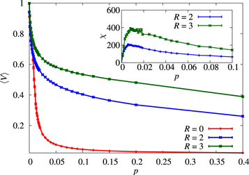
Figure A1. The figure displays the effect of increasing the alignment range using the modified model of equation (A.1). All the data are for  . The curve for R = 0 corresponds to the model previously shown in figure 3. Increasing the alignment range makes it more difficult for the dissenters to completely break the flock, resulting in a slower decay of
  . The effect of just a few dissenters is, however, still very strong and the peak in the susceptibility (i.e., the transition point) hardly moves with respect to the R = 0 case (see inset).
Download figure:
Standard image High-resolution imageAppendix B.: The effect of excluded-volume interactions
Most numerical studies of flocking, starting with the seminal paper by Vicsek et al [1], consider point particles. We have, instead, opted for a model which, in addition to alignment, has excluded-volume interactions, because we believe that this in an important factor for practical applications (such as human crowds), even though it makes simulations harder. In this appendix we briefly explain the qualitative difference between these two kinds of flocking systems.
In order to simulate flocking point particles, we drop the excluded-volume interaction from the modified model presented in appendix A (we need the model with explicit alignment range R since there will be no collisions). That is, aligners will move according to the equations


This is very similar to the model considered in [17].
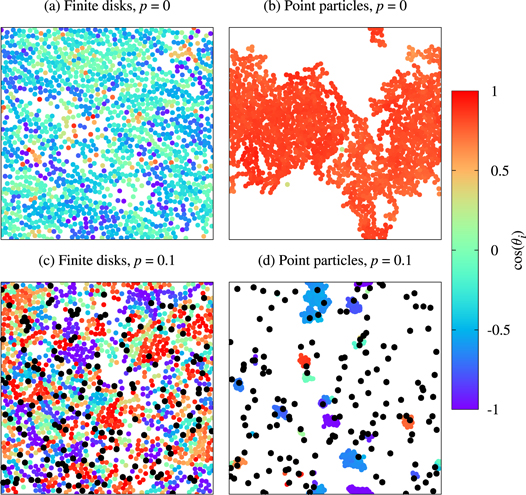
Let us first consider the case p = 0, for which we plot two snapshot of the system in panels (a) and (b) of figure B1. Panel (a) considers the case with particle radius a = 1, just like in the rest of the paper. Since there are no dissenters the particles are moving in basically the same direction, with some small deviations due to occasional random collisions. Crucially, the disks are distributed essentially homogeneously throughout the simulation box. In panel (b), on the other hand, we show an equal number of flocking point particles. The configuration is now very different: since there is nothing to keep the particles apart, the flock is much more concentrated and the local density is very heterogeneous. In fact, the flock is starting to form a well-defined band, as has been widely reported for the Vicsek model (see, e.g., [8]).
Figure B1. Comparison of the system's behavior with and without excluded volume interactions. We show snapshots of steady-state configurations for four cases. The left column of plots, panels (a) and (c), consider self-propelled disks of radius a = 1, just as in the rest of the paper. Each disk is plotted with a color given by its instantaneous orientation (the packing fraction is  ). In panel (a), there are no dissenters (p = 0) and most particles have the same orientation. In panel (c), on the other hand, we have introduced a fraction p = 0.1 of dissenters (in black) and the system is disordered, as shown by the very different disk colors. The right column considers analogous cases, but now for an equal number of point particles (which are nevertheless plotted as disks for comparison purposes). Panel (b) shows the pure system, with a very ordered flock that, unlike in panel (a), is forming a band. In panel (d), the dissenters have caused the aligners to aggregate in several small and very concentrated clusters. In all cases we have used the modified model of appendix A with R = 2.
Download figure:
Standard image High-resolution image
Once we introduce dissenters, the differences between finite disks and point particles become even more striking. On panel (c) of figure B1 we show a snapshot of the system with excluded volume and a high concentration of dissenters (p = 0.1). Now there is no flock, but the excluded-volume interactions still force the particles to space themselves uniformly. Panel (d) shows the corresponding configuration for the same number of point particles and p = 0.1. Now the dissenters have forced the aligners to aggregate in tiny but very concentrated clusters, each moving in a random direction, while the dissenters themselves are naturally still distributed uniformly throughout the system.
Notice that this comparison explains why, unlike in [17] or recent studies of the flocking transition in the Vicsek model, we find scale invariance at the transition, since the steric repulsion prevents concentrated bands of particles from forming and keeps density fluctuations small.
Appendix C.: Hydrodynamics of a mixture of aligners and dissenters
Here we derive the hydrodynamic equations for aligners and dissenters using a continuous-time Vicsek model of point particles. The model contains two simplifications as compared to the one used in simulations: (i) we neglect excluded volume interactions among the particles; and (ii) aligners align with the orientation of neighboring particles, instead of aligning with their own direction of motion. These simplifications allow us to carry out the derivation of the continuum equations analytically. Note that the findings of appendix A indicate that the details of the alignment affect the dynamics only quantitatively, but not qualitatively.
C.1. Derivation of the continuum equations
Aligners are located at positions  for
for  and are self-propelled at speed v0 in the direction
  . Likewise, dissenters located at positions
  , for
, for  , have self-propulsion speed vD along
  . Aligners align with each other and also with dissenters, whereas dissenters cannot align. The dynamics of the system is governed by
The alignment couplings have the form  , which describe contact interactions between particles of size a. This determines a range of interaction comparable to that of our simulations. As in the numerical model discussed in section 2,
  are stochastic terms describing white noise with correlations
  .
.
We introduce the one-particle density of aligners (dissenters) describing the probability of finding an aligner (dissenter) at position  (
( ) moving in the direction
  (
( ) at time t as

The continuum equations for aligners and dissenters can be derived by coarse-graining the microscopic equation (C.1), following a standard procedure (see, e.g., [32]). First, one obtains noise-averaged Smoluchowski equations for both aligners and dissenters of the form
To obtain equations for density and polarization we now consider the angular moment of the probability densities, given by

with  labeling aligners or dissenters. We indicate complex conjugated using an overbar. The first few moments are related todensity and polarization density, with

denoting for simplicity the zeroth moments by ρ and  , the equations for the first few moments of the aligners density are given by
where we have defined  and
and  Similarly, for the dissenters we obtain
As discussed in [36], a consistent approximation for a system with polar symmetry is obtained by neglecting all moments of order equal to or higher than n = 3 and noting that the second moment  is proportional to the component of a nematic order parameter that in a system with polar interactions decays on microscopic time scales even in the ordered flocking state. We therefore neglect
  in equations (C.5) and (C.6) and eliminate
  from the dynamics using
Replacing these expressions in equations (C.5) and (C.6) we obtain a closed system of equations for  and
and  which result in the set of hydrodynamic equations, equation (12) of the main text.
C.2. Correlation functions
To evaluate the correlation function of polarization fluctuations, we linearize the hydrodynamic equations deep in the flocking state by letting  ,
,  ,
,  and
and  , with
  . We set
  . and write
 ![$\delta {\boldsymbol{P}}=[\hat{{\boldsymbol{x}}}\delta P+\hat{{\boldsymbol{y}}}{P}_{0}\delta \theta ]$](https://content.cld.iop.org/journals/1367-2630/19/10/103026/revision2/njpaa8ed7ieqn160.gif) . Keeping terms to linear order in the fluctuations in equation (12) and eliminating
. Keeping terms to linear order in the fluctuations in equation (12) and eliminating  in favor of
  yields
with ![${v}_{1}={v}_{0}{\rho }_{0}\alpha ^{\prime} ({\rho }_{0})/[2\alpha ({\rho }_{0})]\simeq {v}_{0}$](https://content.cld.iop.org/journals/1367-2630/19/10/103026/revision2/njpaa8ed7ieqn163.gif) , where the second equality holds deep in the flocking state. We evaluate correlation functions in Fourier space by introducing the Fourier amplitudes of the fluctuations,
, where the second equality holds deep in the flocking state. We evaluate correlation functions in Fourier space by introducing the Fourier amplitudes of the fluctuations,  , for any function g. The angular correlations are then given by

where we let  . The equations for the dissenters are decoupled form those of the aligners. The correlation function of the fluctuations in the dissenters' polarization density is then easily calculated, with the result

where  . The equal-time correlation is given by
  , with the result

The first term on the right hand side of equation (C.11) are the fluctuations in the pure system, the second one is the contribution for the dissenters. In the long wavelength limit, and using that  , equation (C.11) can be rewritten as equation (15). In other words the presence of dissenters essentially renormalizes the noise strength.
Finally, for comparison we note that static obstacles could be incorporated in the continuum model by quenched disorder corresponding to a stochastic force in equation (C.9) of the form  , obtained as the gradient of a random potential ϕ (see, e.g. [12]) and with correlations
  . Using this expression in equation (C.9) and considering the limit
  as in [12], one obtains the result presented in the main text, equation (16).